机器学习-炮哥带你学入门
教程地址:
- up:炮哥带你学
课程名字:[手把手教学]快速带你入门深度学习与实战
简介:入门机器学习和深度学习
网址:
- up:炮哥带你学
课程名字:Pytorch框架与经典卷积神经网络与实战
简介:入门深度学习和pytorch
网址:
简介
深度学习以神经网络为基础
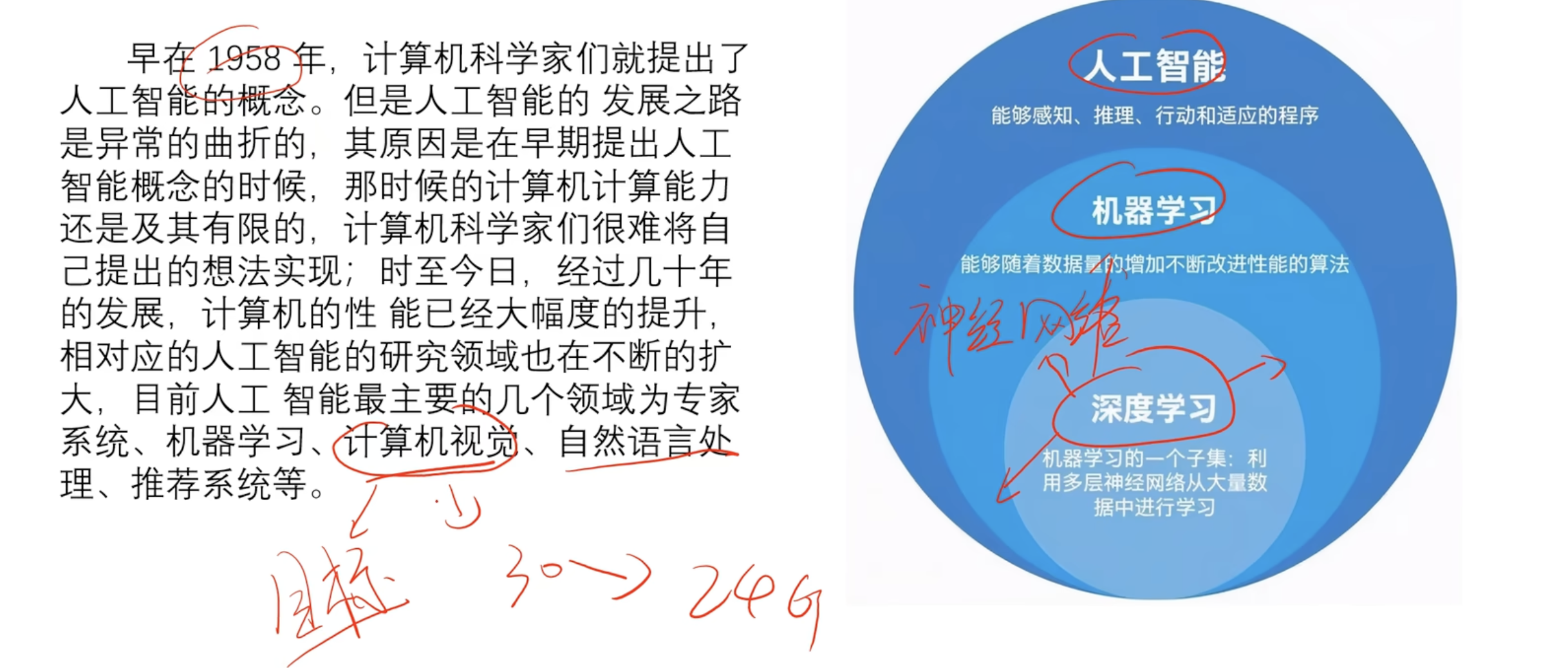
神经网络
- 并非隐藏层越多越好 可能过拟合
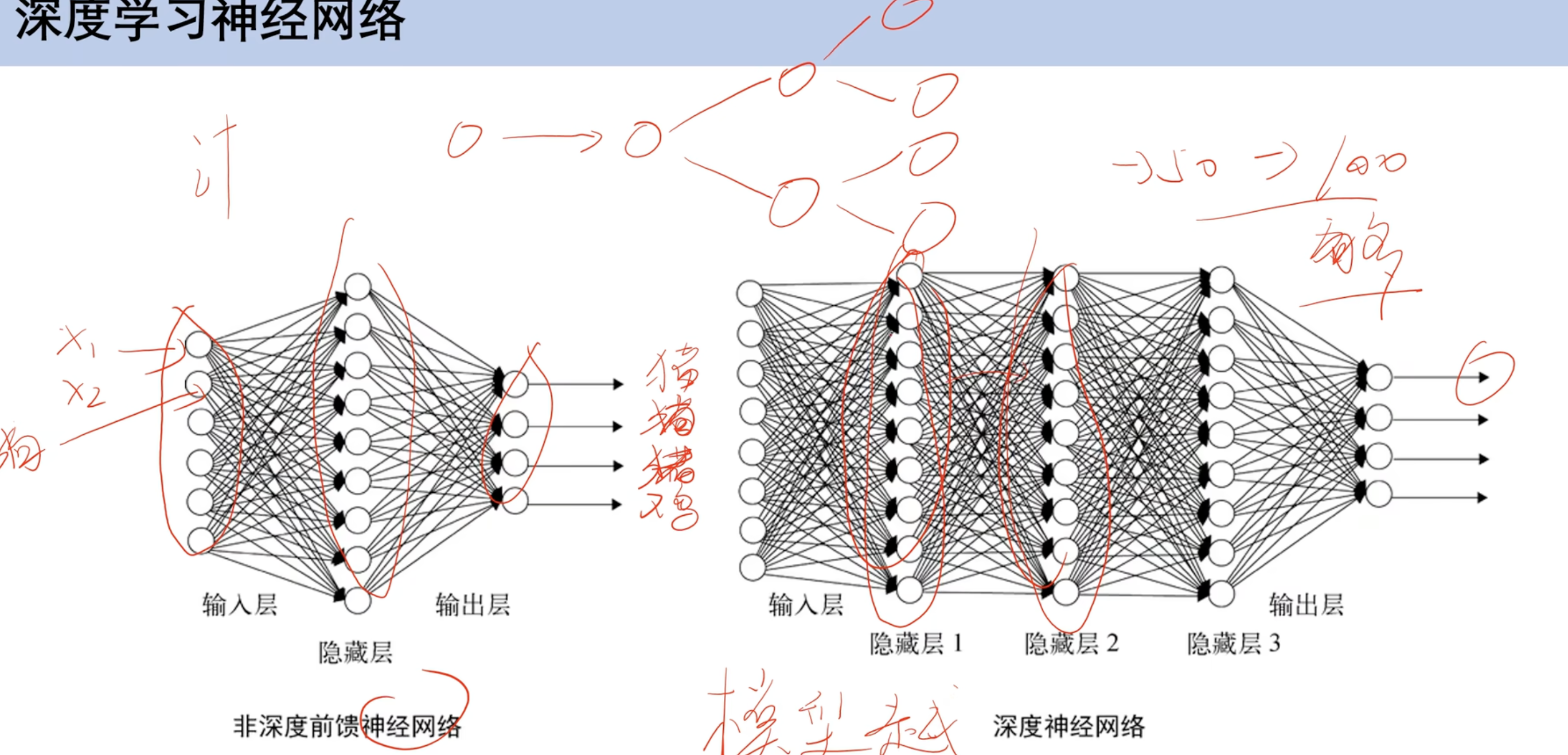
全连接神经网络
通过训练w和b(权重和偏置)
- 注:机器学习内容
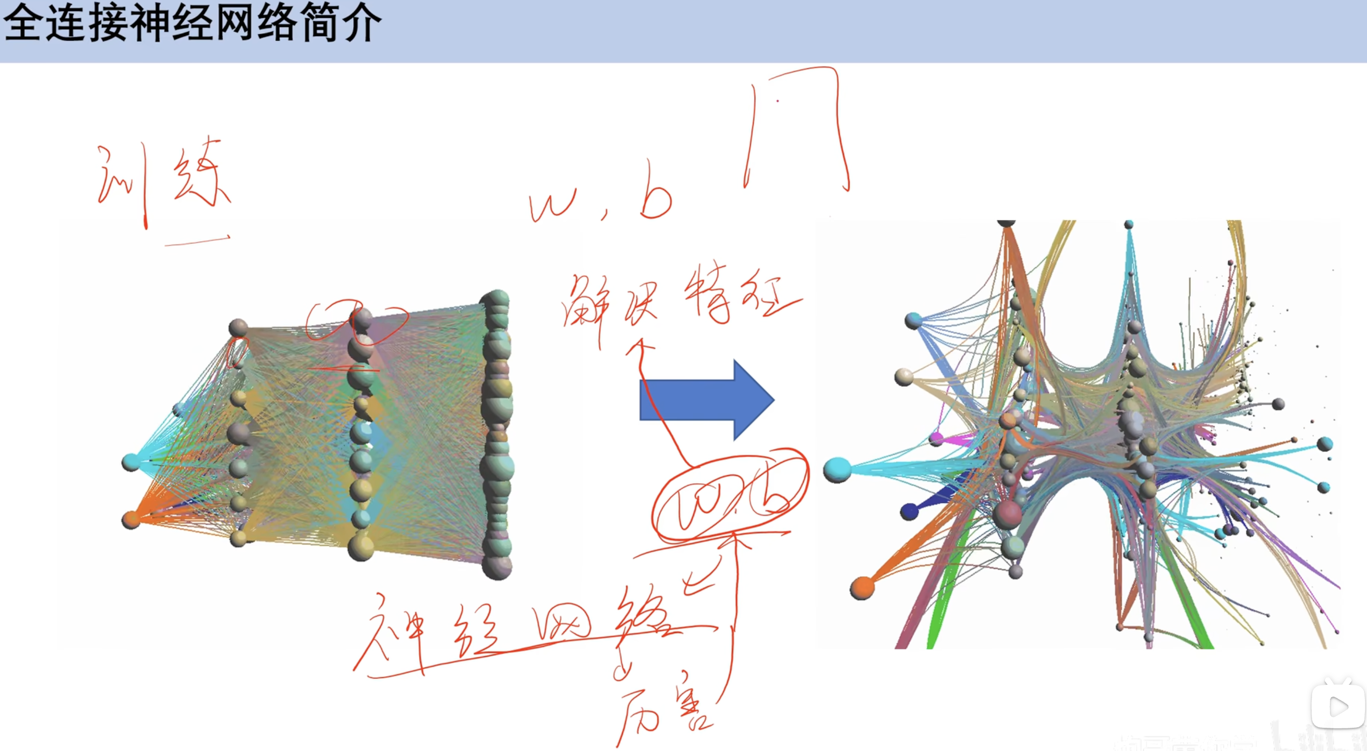
神经网络作用
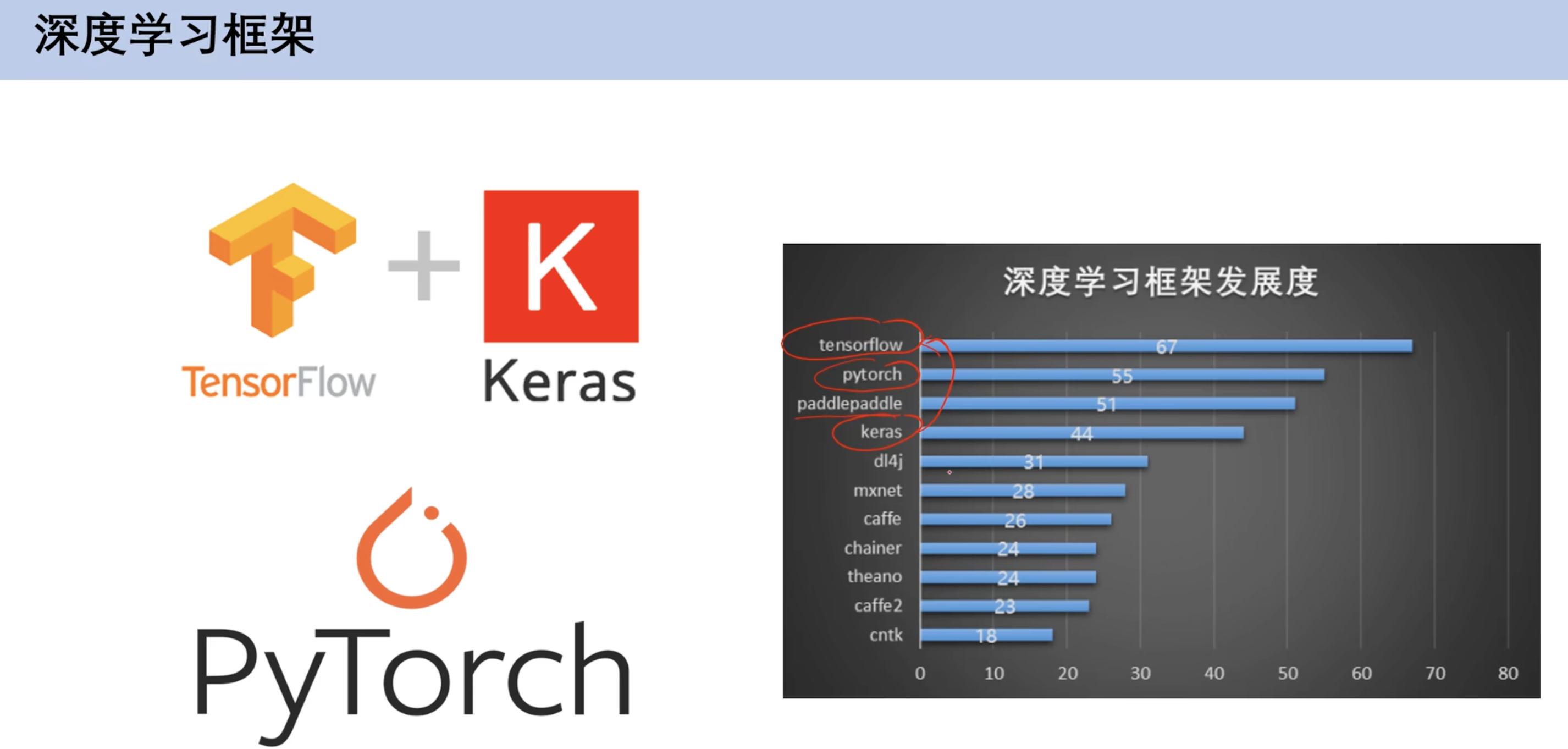
==深度学习框架介绍==
环境介绍

机器学习知识回顾
2. 线性回归模型与梯度下降
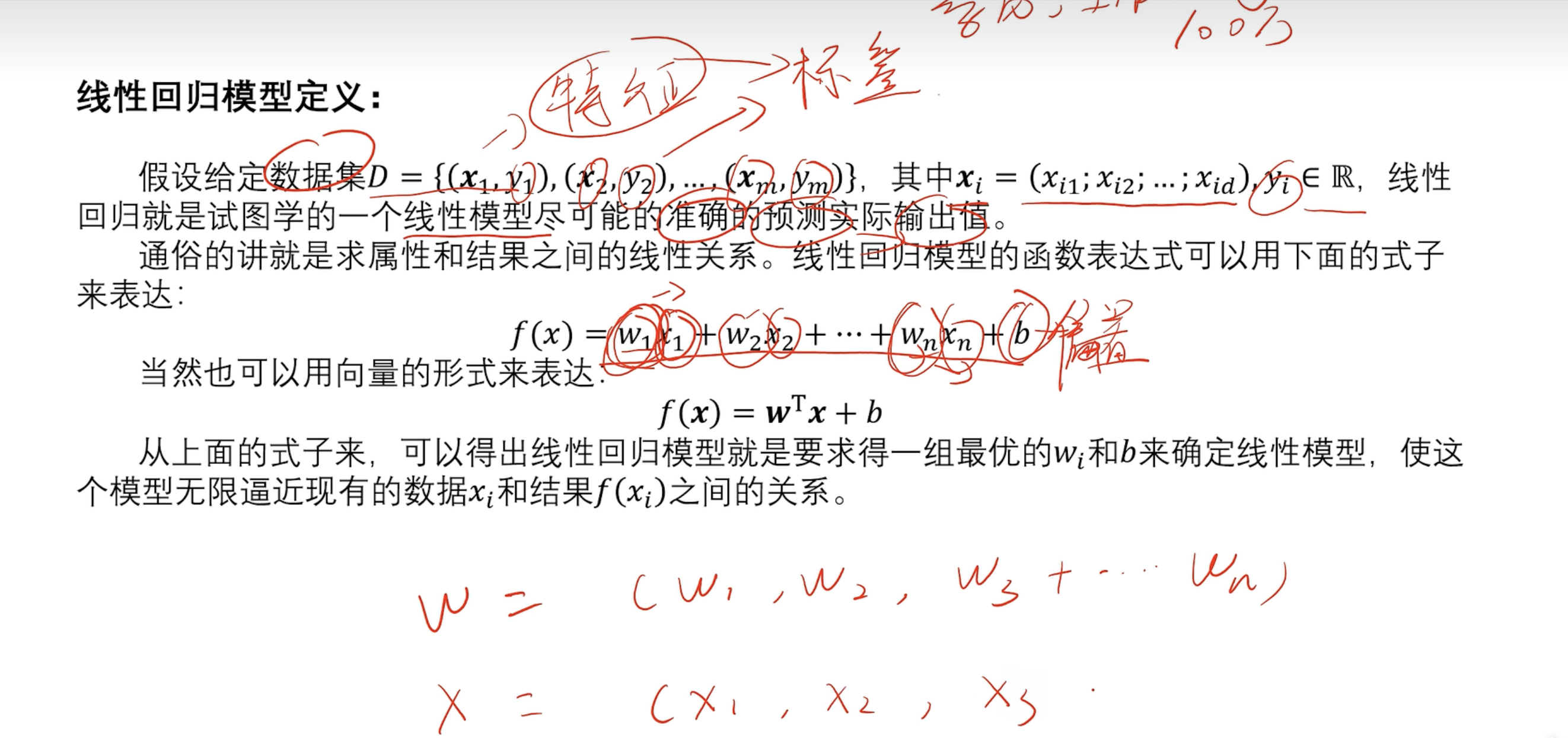
2.2 定义
- x是特征 y是标签
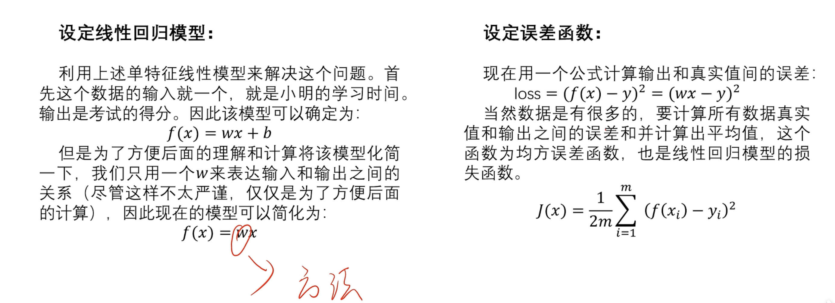
损失函数 (误差函数)
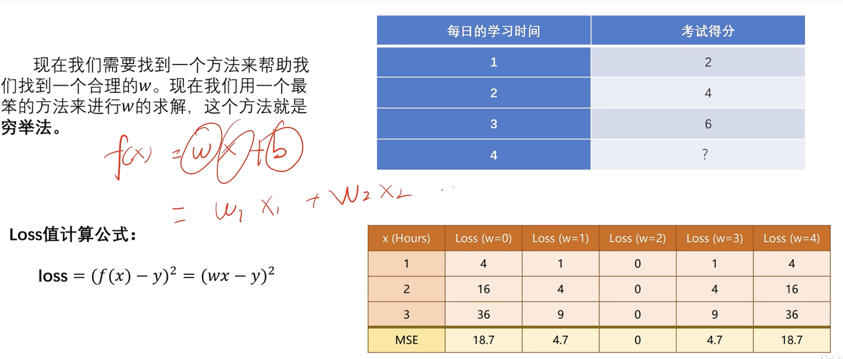
穷举法
- 过于垃圾 看后面最小二乘法
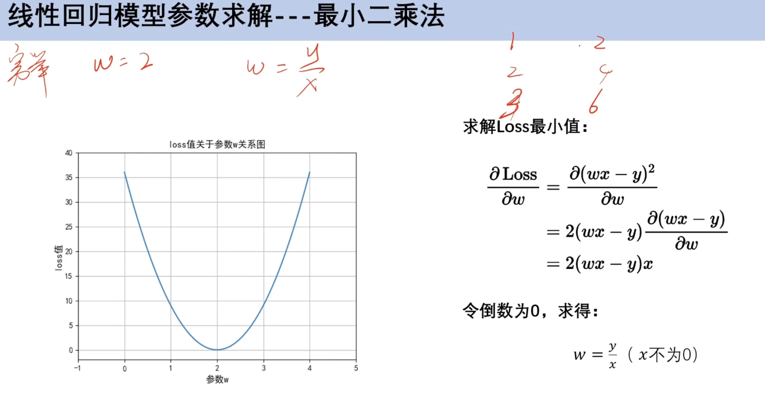
2.3 最小二乘法
对x求偏导
向量版本
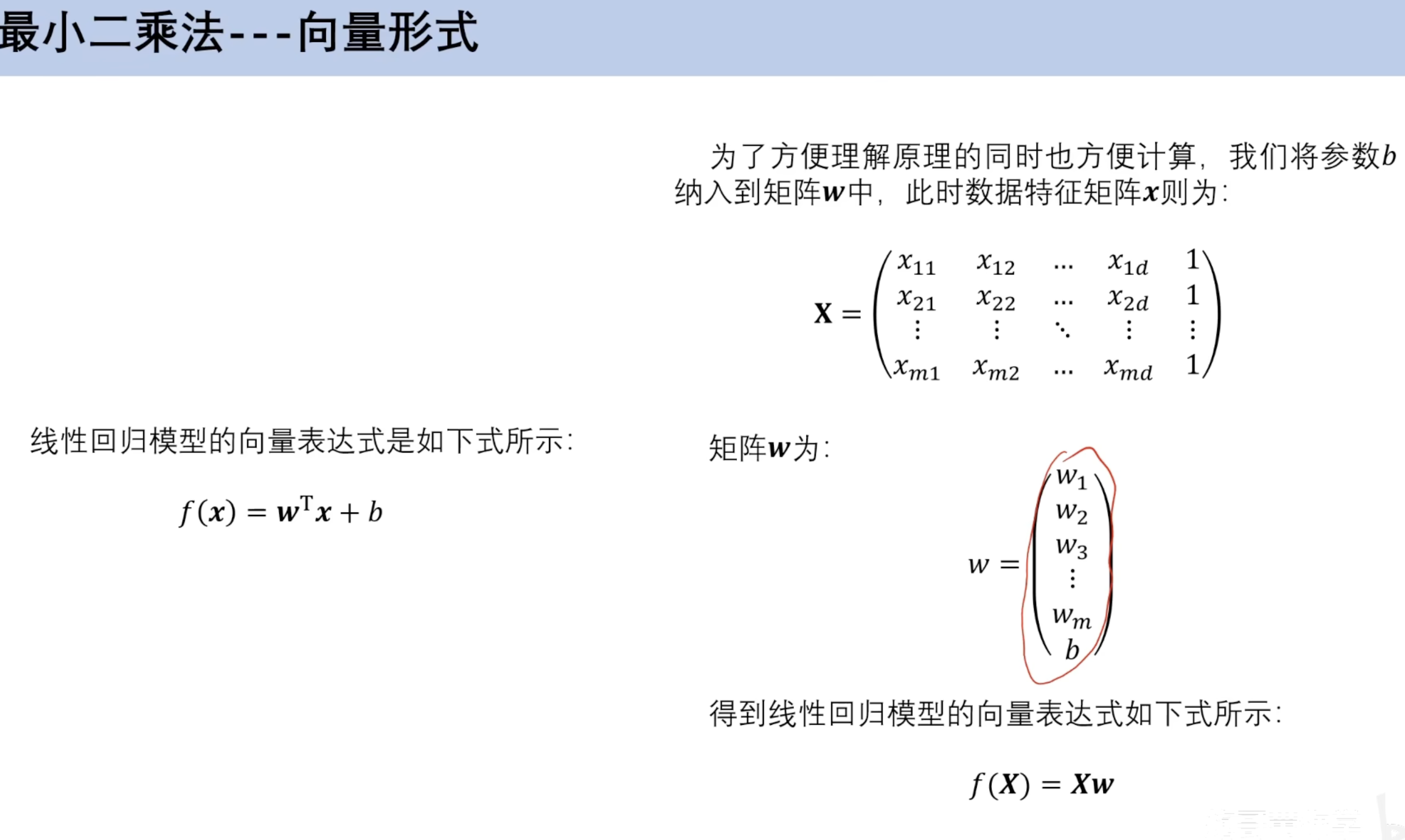
- 损失函数
- 更正 此处J(W)为f(x)
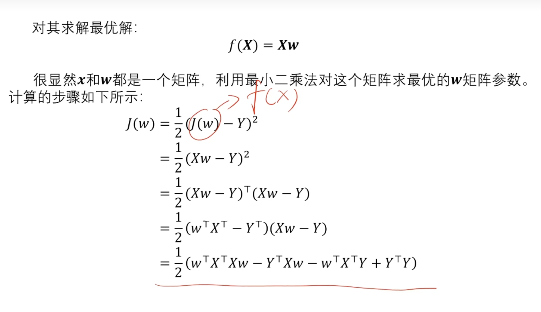
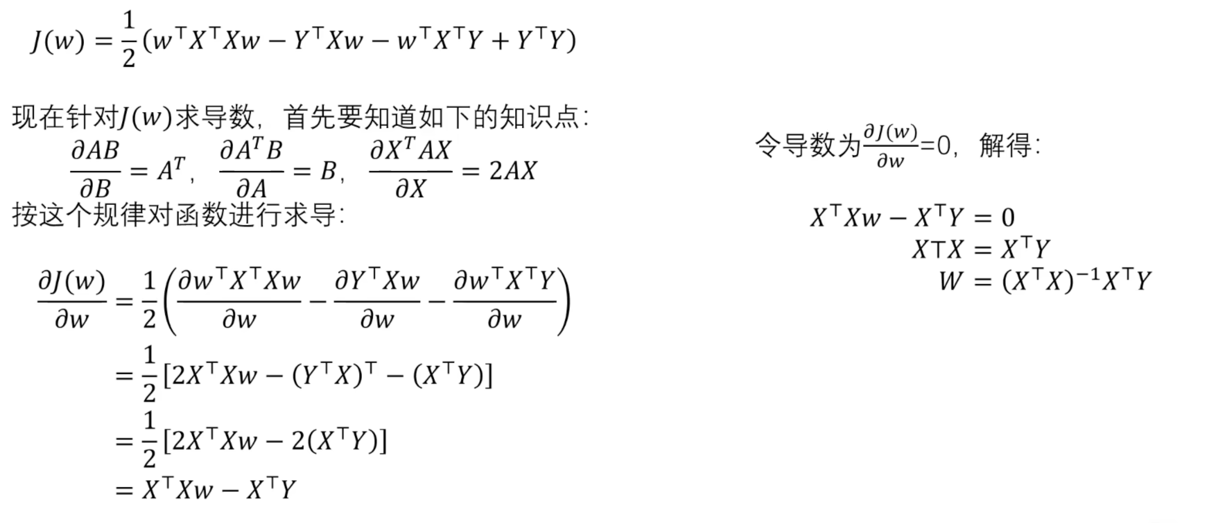
- 对损失函数求导
并非所有矩阵有可逆矩阵,因此引入损失函数
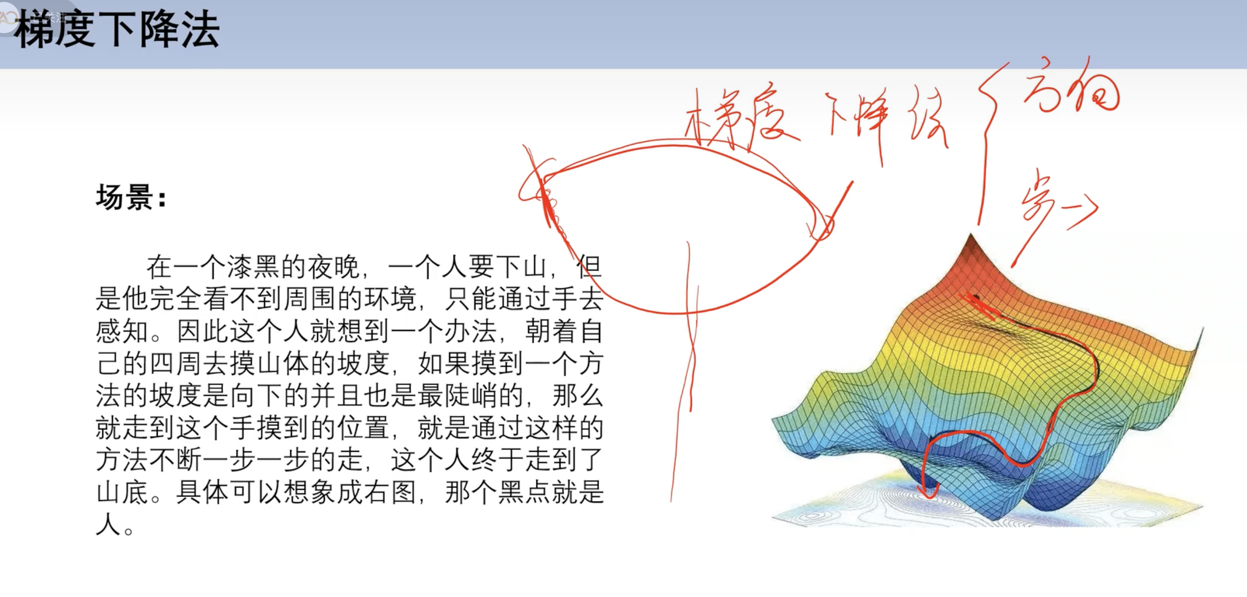
==2.3 梯度下降==
理解
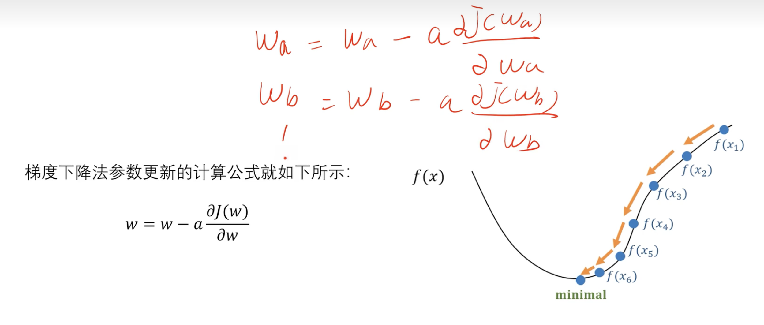
公式
$$
w=w-a \frac{\partial J(w)}{\partial w}
$$
- 对多个w重复计算
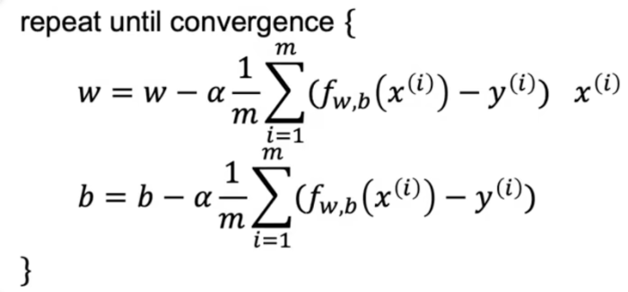
简化版本
$$
\begin{array}{l}
\text { repeat until convergence { }\
\begin{aligned}
w & =w-\alpha \frac{1}{m} \sum_{i=1}^{m}\left(f_{w, b}\left(x^{(i)}\right)-y^{(i)}\right) x^{(i)} \
b & =b-\alpha \frac{1}{m} \sum_{i=1}^{m}\left(f_{w, b}\left(x^{(i)}\right)-y^{(i)}\right)
\end{aligned}
\end{array}
$$
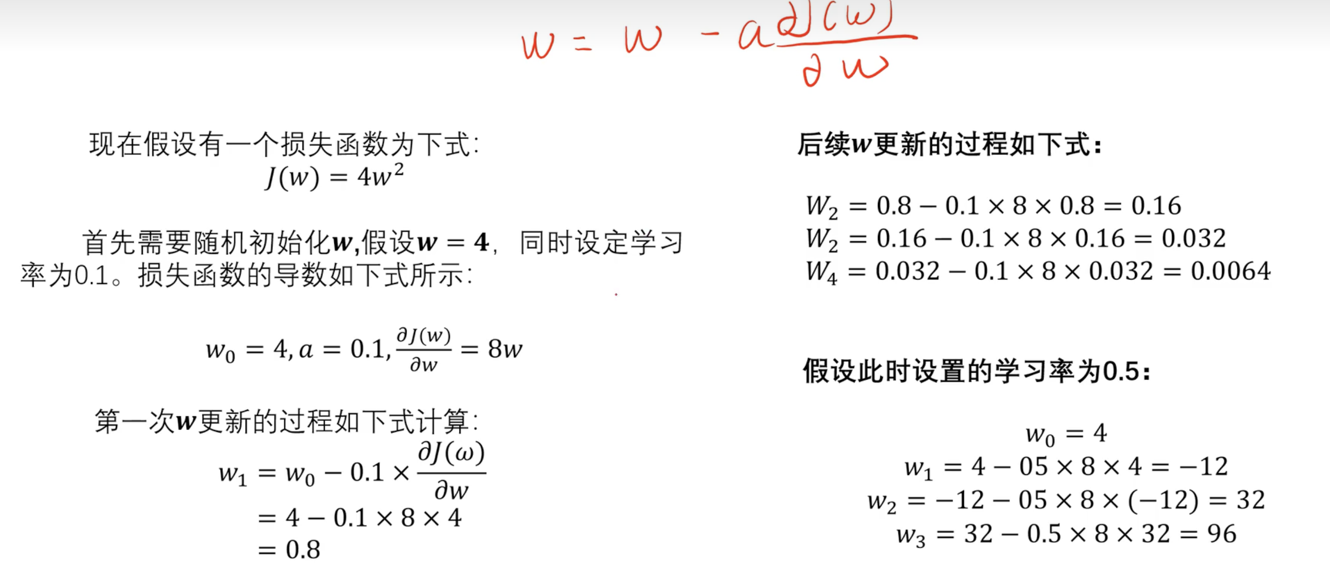
案例
实战案例
步骤:
- 数据
- 模型
- 损失函数
- 梯度求导
- 利用梯度更新参数
- 设置训练轮次
1 | # 定义数据集 |
==3.逻辑回归==
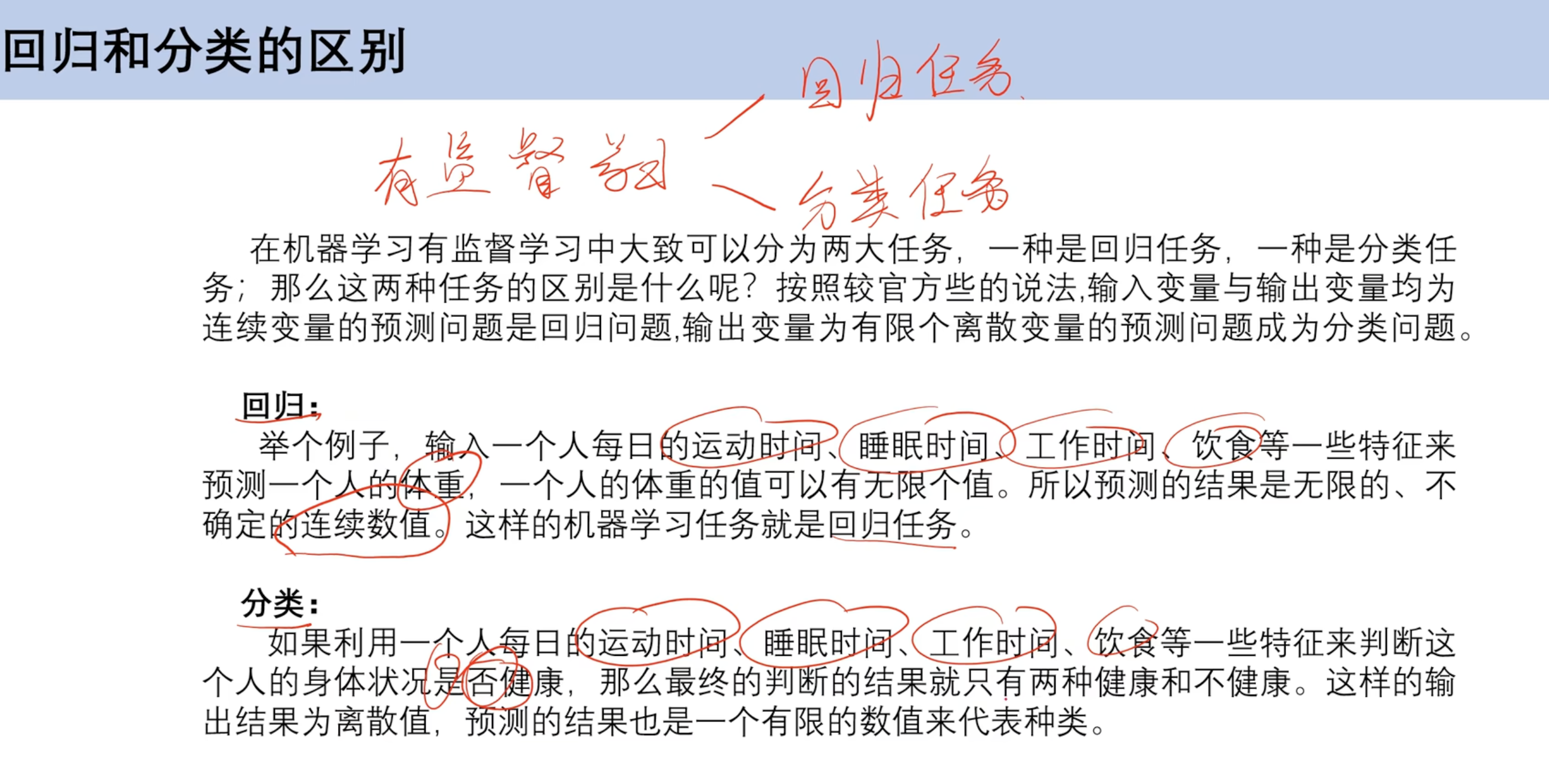
3.1 回归和分类的区别
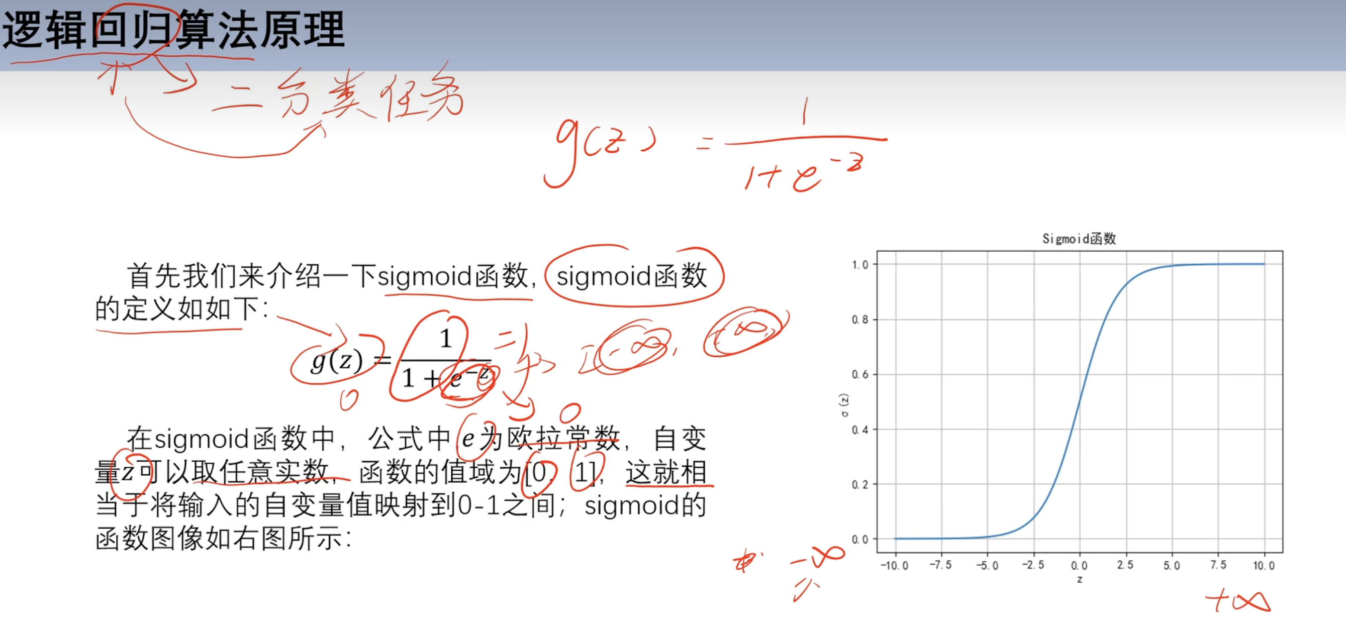
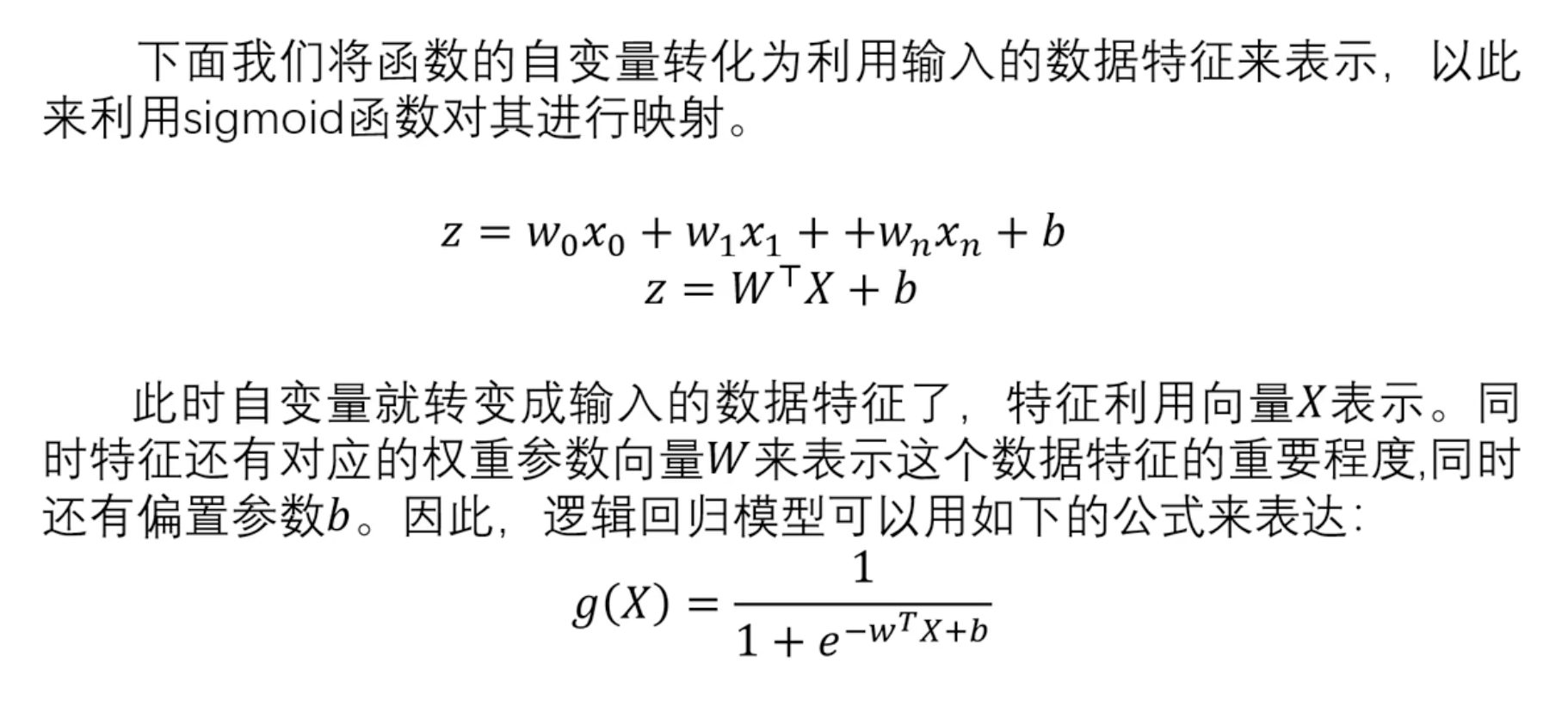
3.2 sigmoid函数
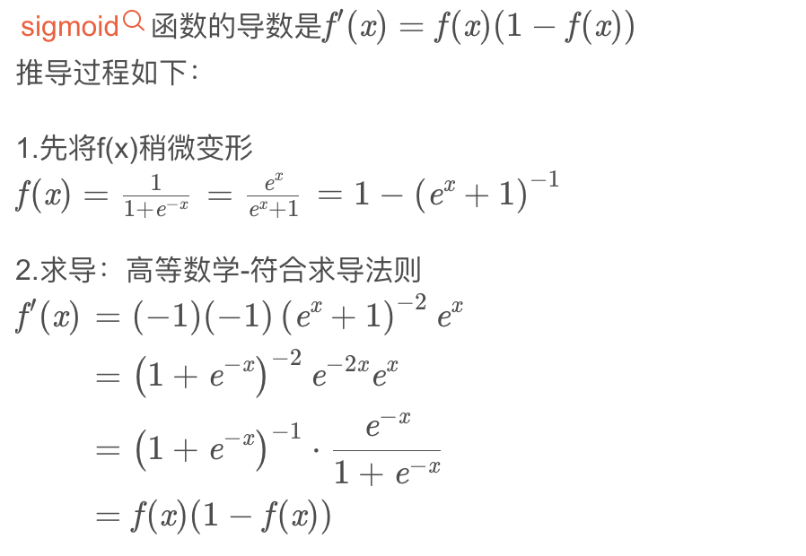
求导
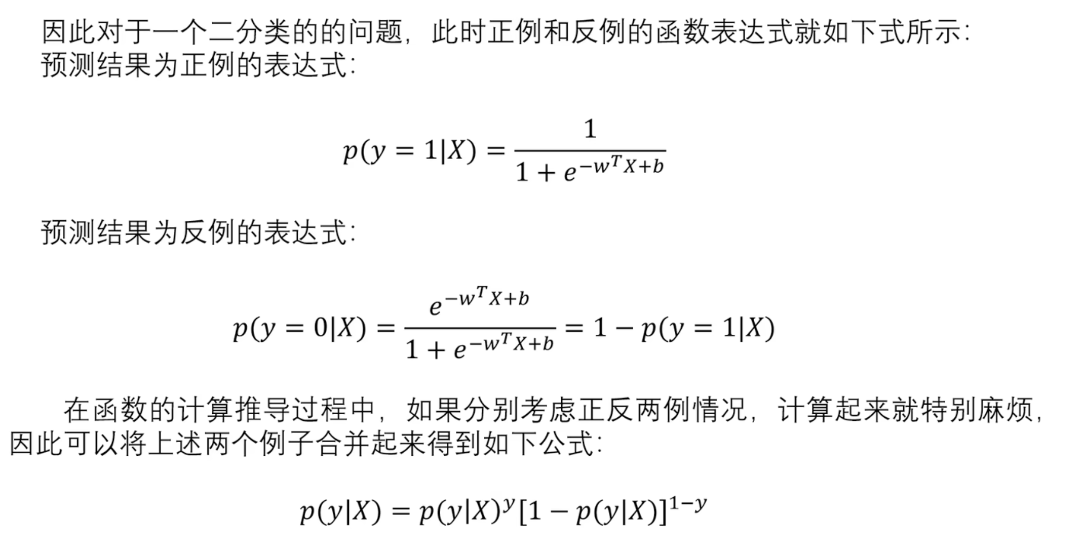
==3.3 损失函数==
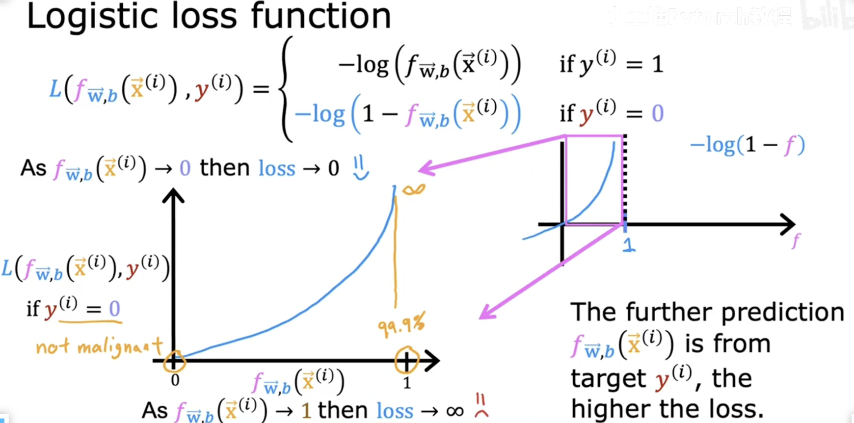
表达式
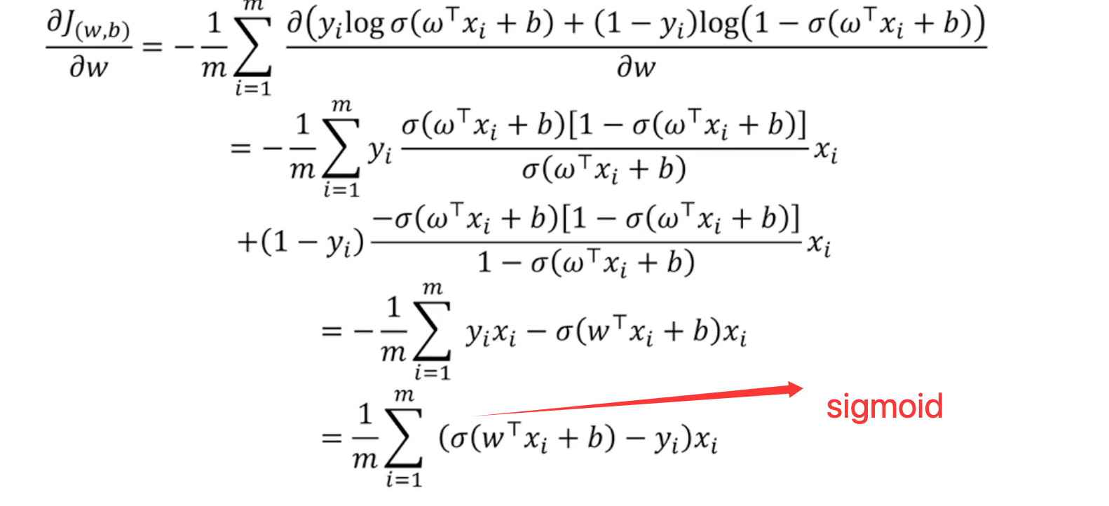
==3.4 梯度下降==
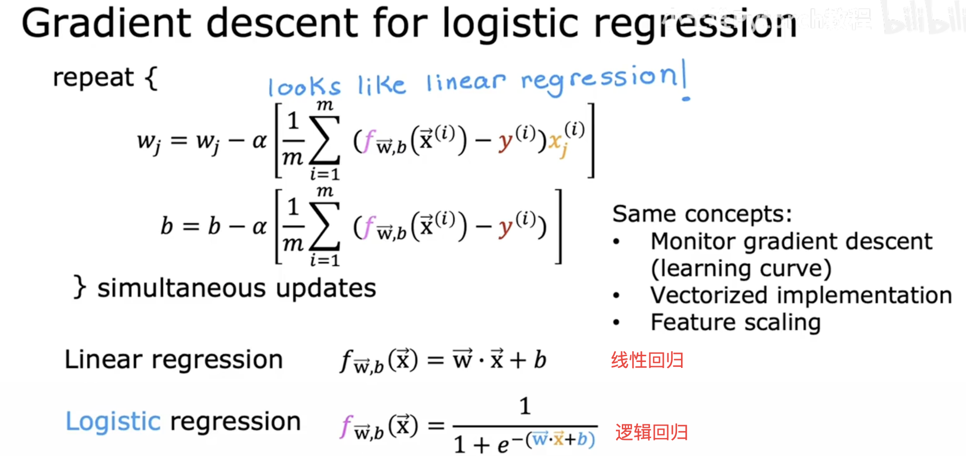
参数w更新

- 向量求导
- 带入函数常规求导推导:
参数b更新
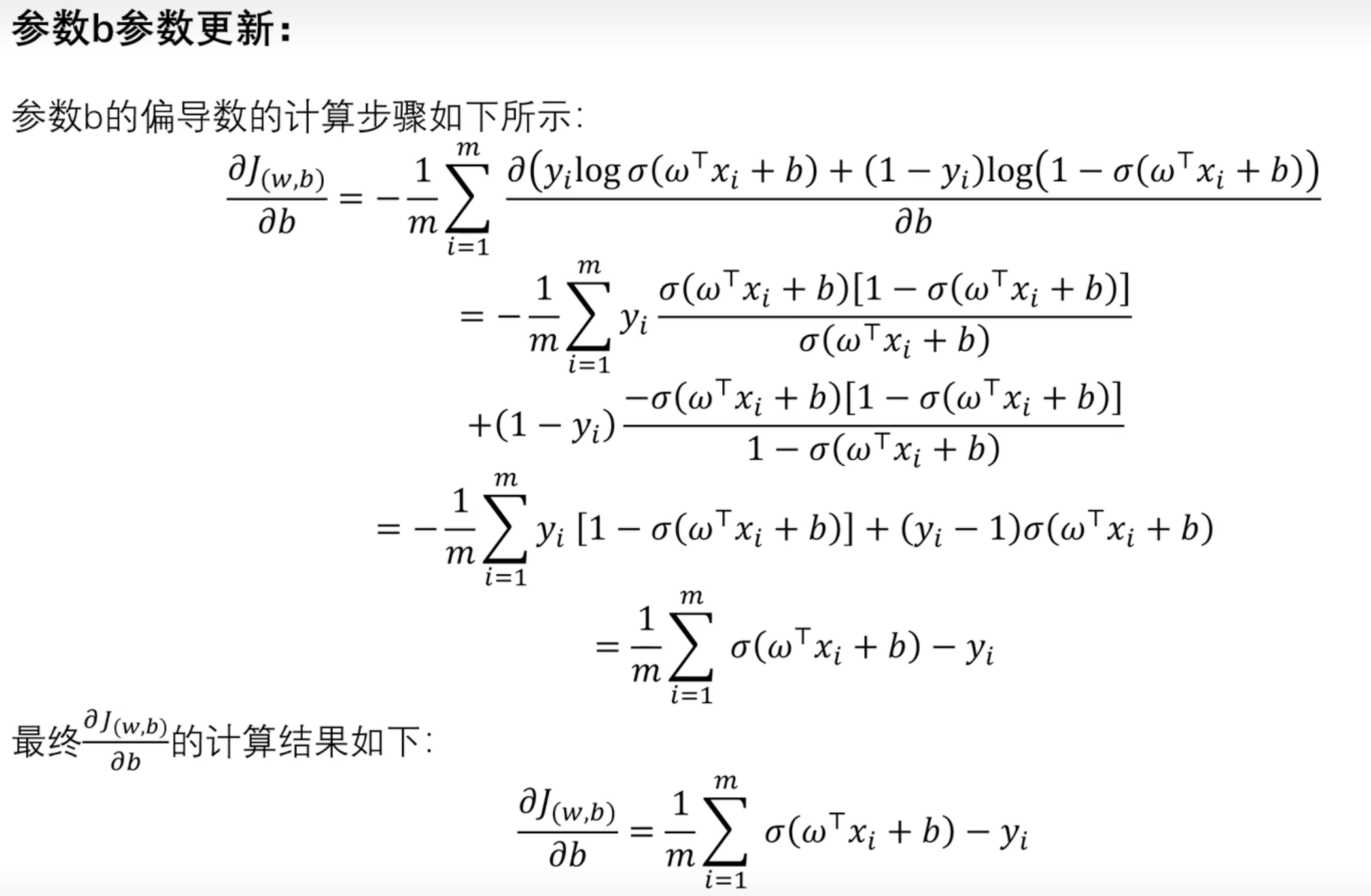
3.5 回归模型评价指标
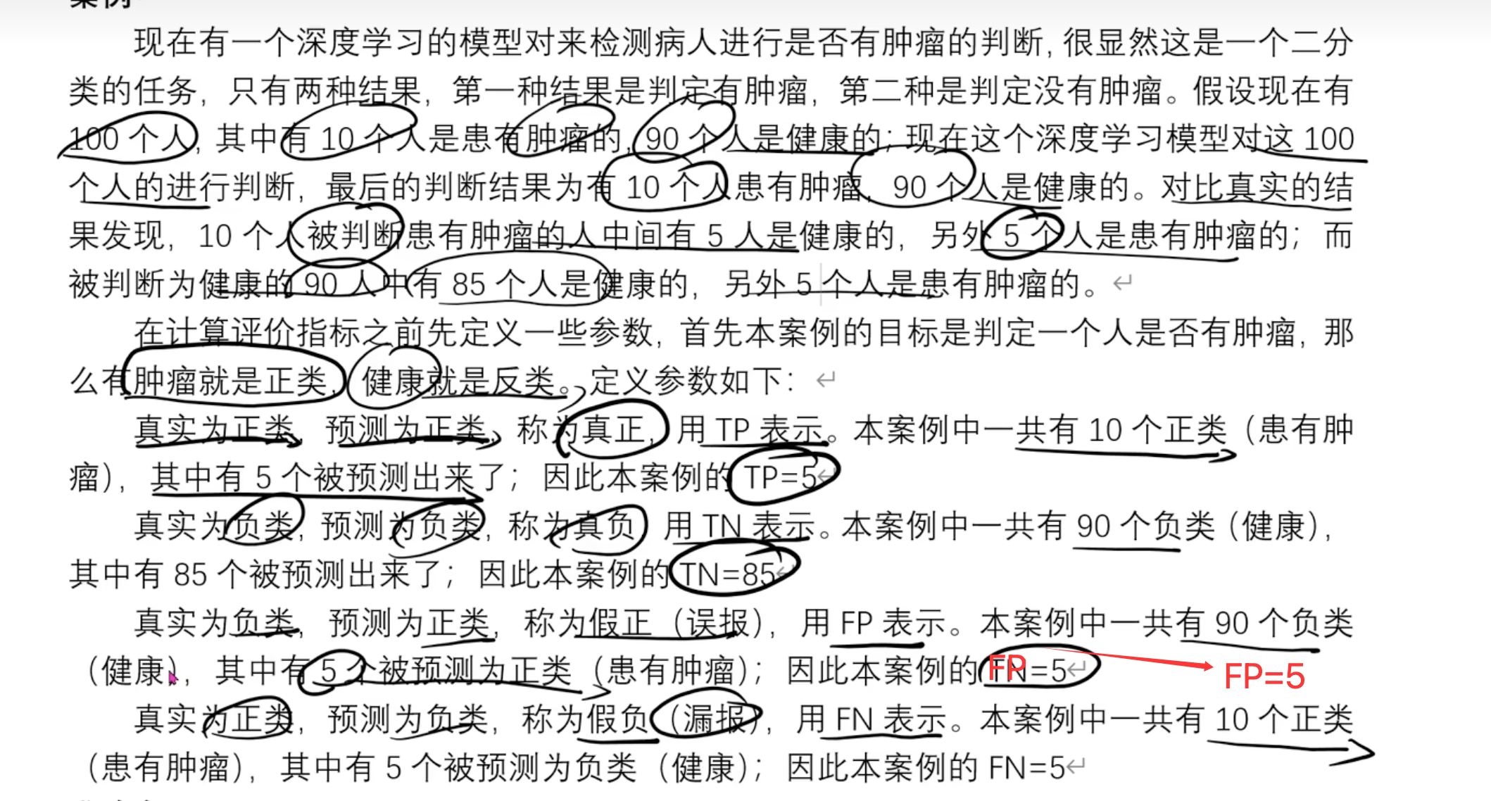
案例
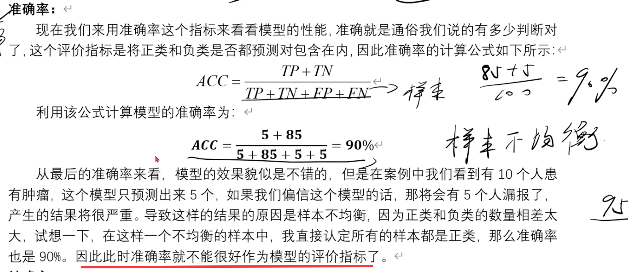
准确率
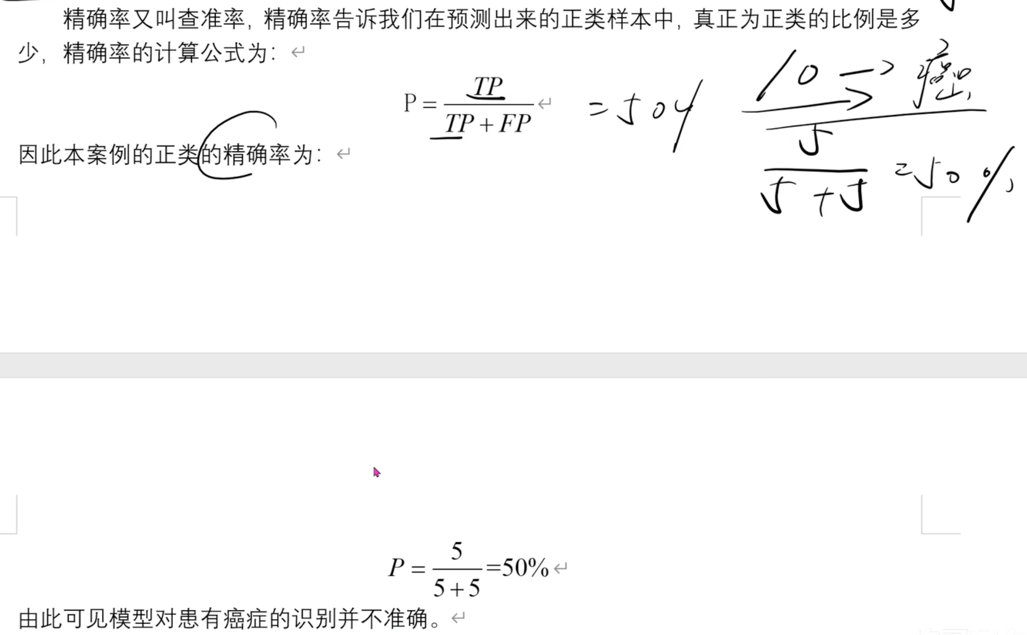
精确率
召回率
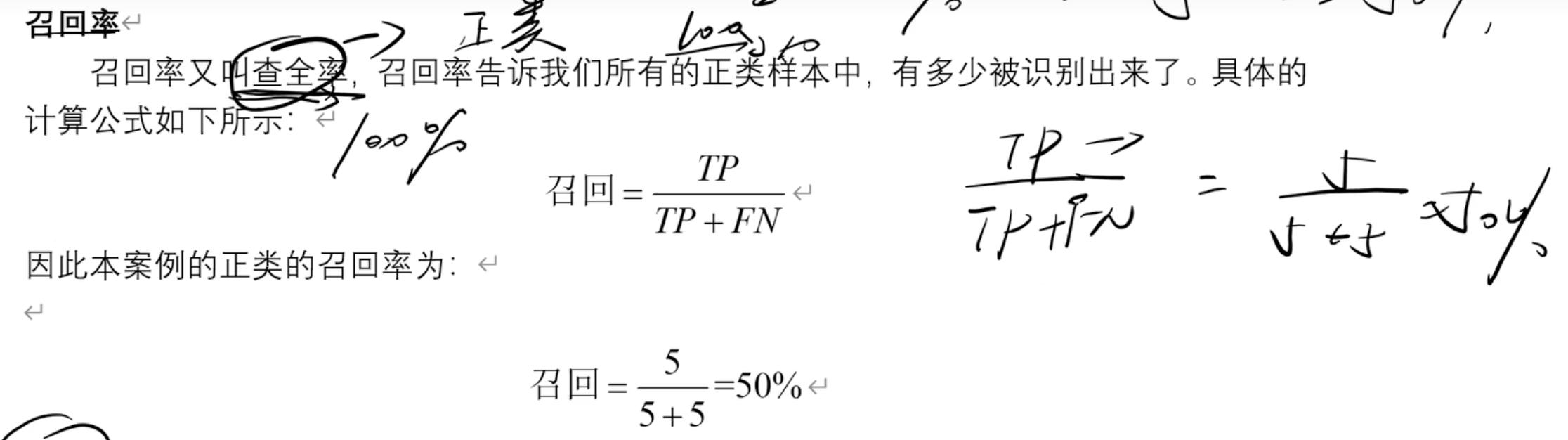
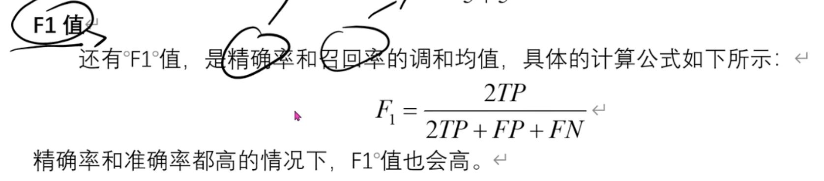
F1值
3.6 分类模型评价指标
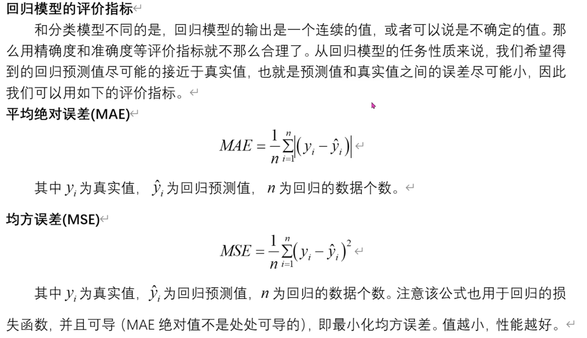
平均绝对误差(MAE)和==均方误差(MSE)==
MSE 就是前面的LOSS 损失函数
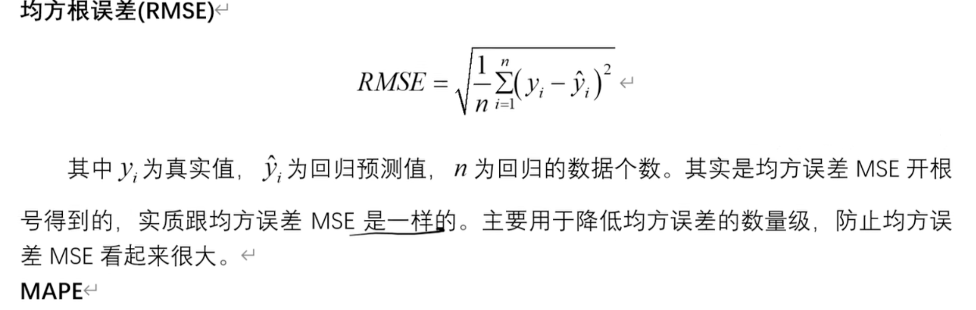
均方根误差(RMSE)
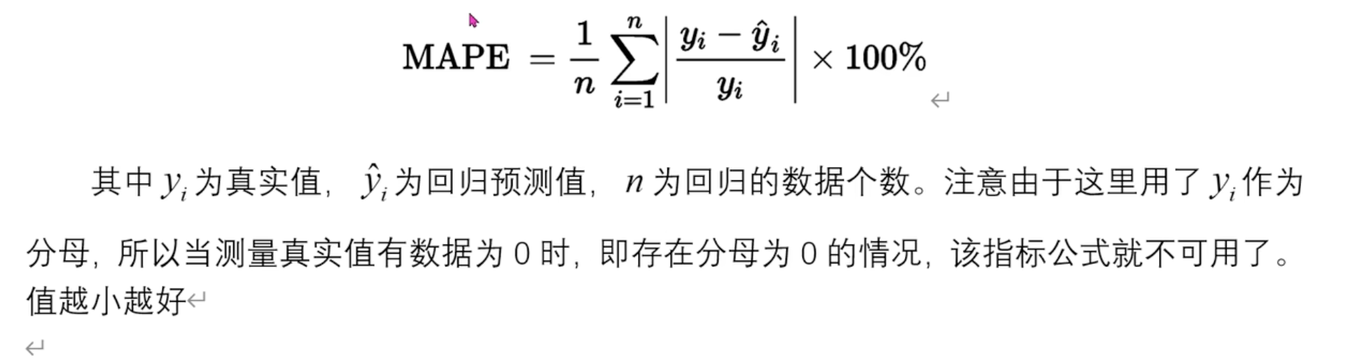
平均绝对百分比误差(MAPE)
3.7 实战案例
代码
- 归一化公式:(X-min)/(max-min),消除量纲和数值大小对结果的影响
1 | import numpy as np |
结果打印
深度学习
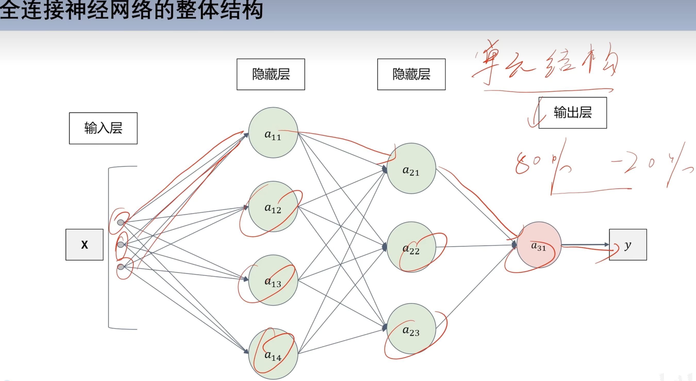
全连接神经网络
结构
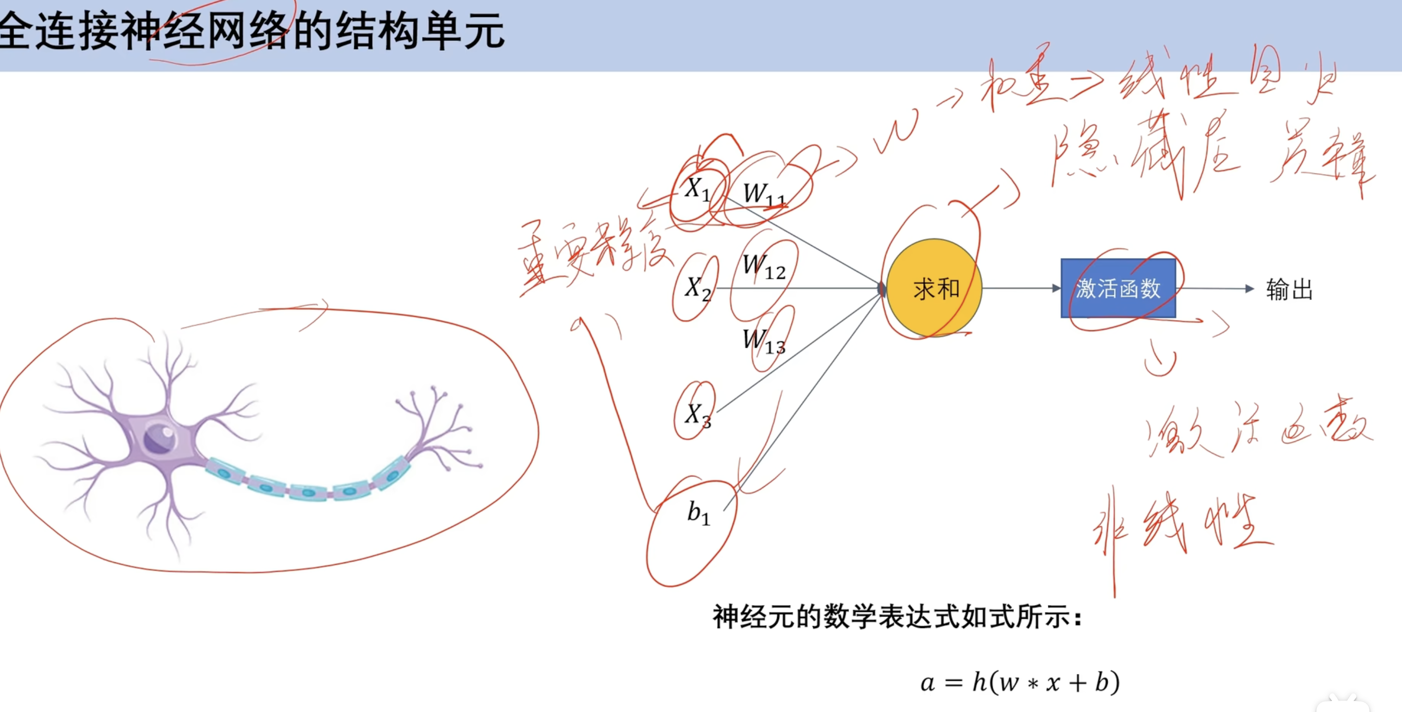
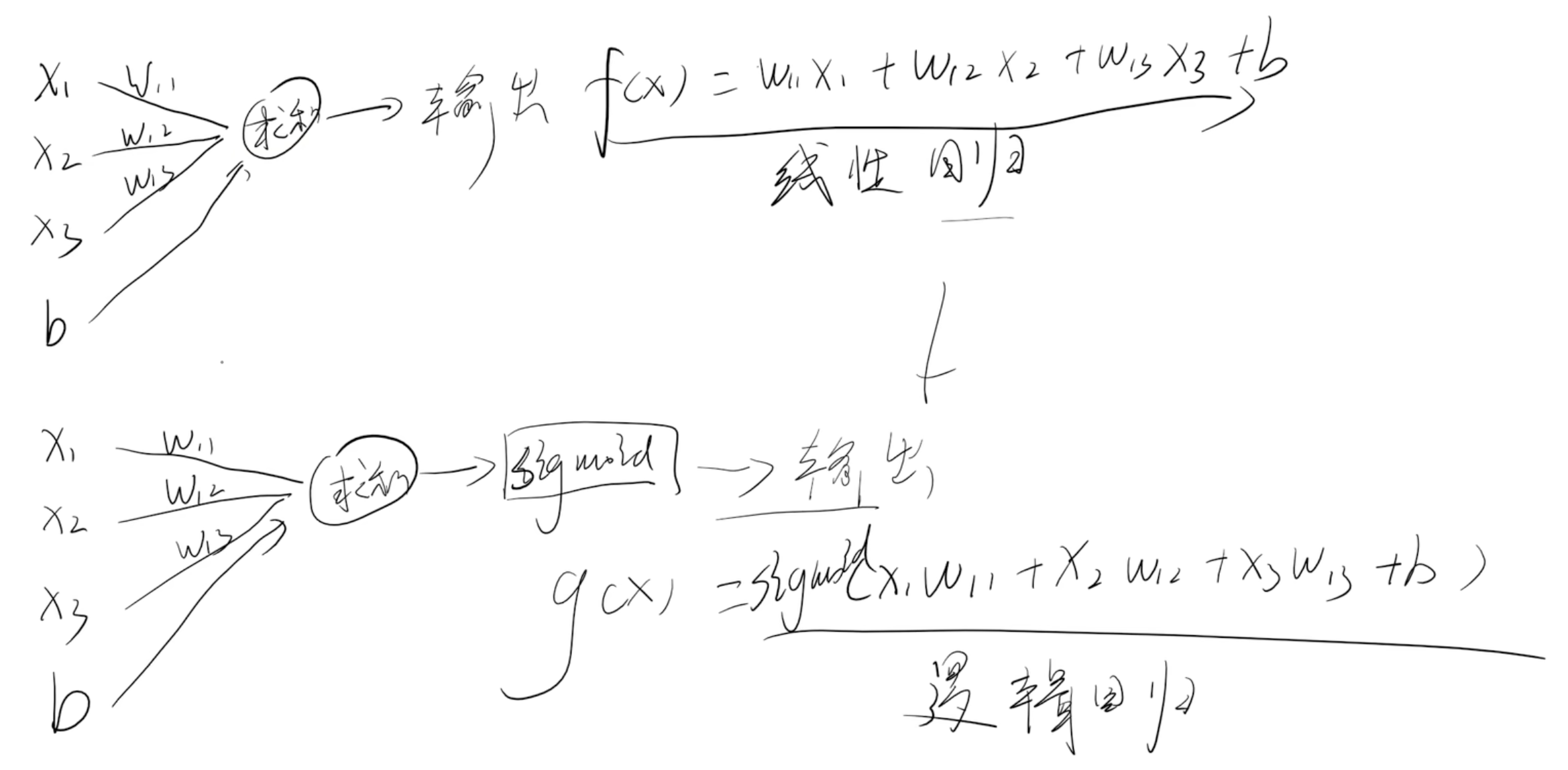
结构单元
- 类比机器学习回归模型
- x 输入
- b 偏置
- w权重
- 求和:隐藏层
- 激活函数:非线性 ==(对比逻辑回归激活函数是求和 逻辑回归激活函数是sigmoid)==
对比机器学习激活函数
对比逻辑回归激活函数是求和 逻辑回归激活函数是sigmoid)
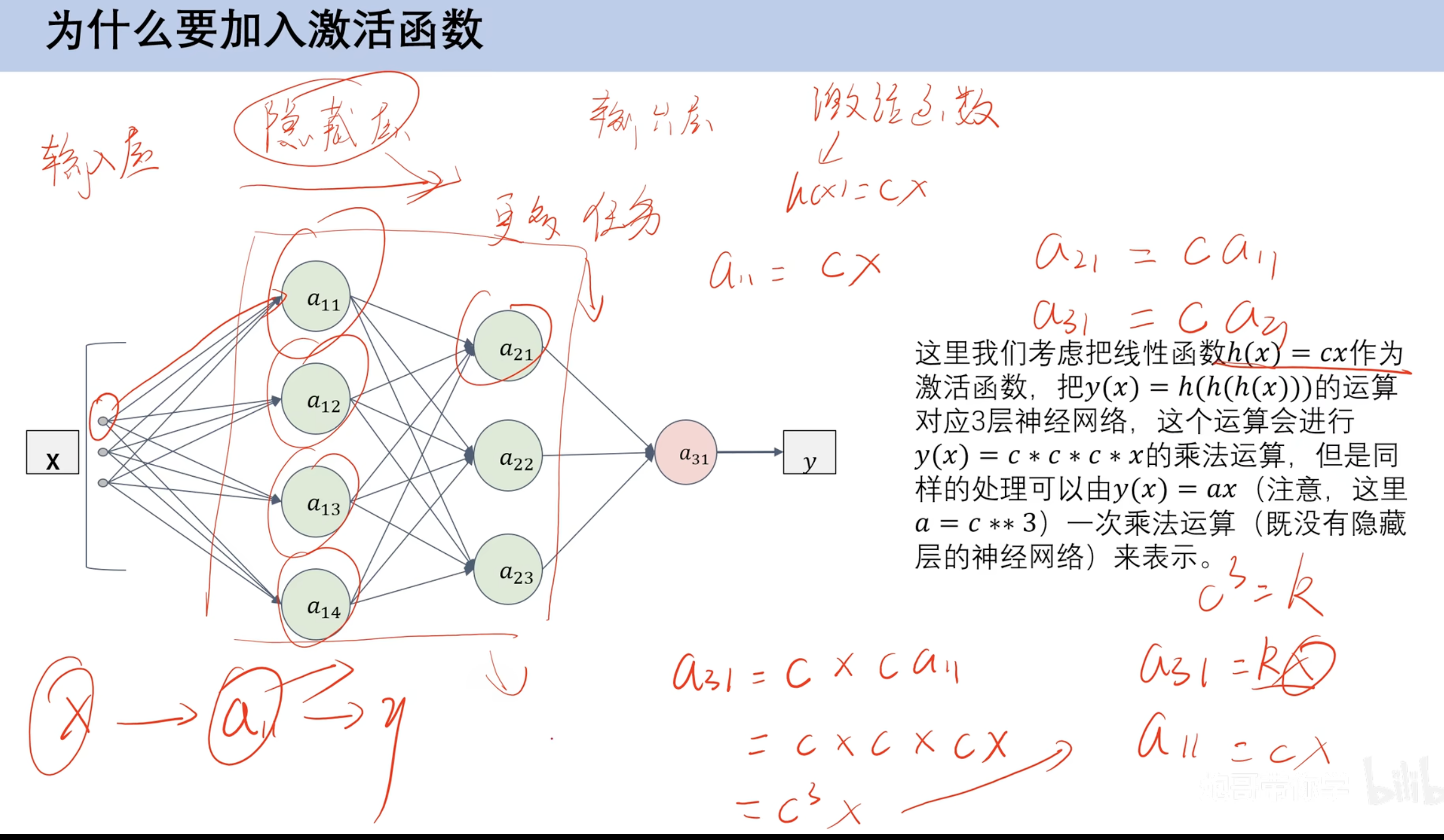
激活函数作用
- 非线性:
这样最后就不会得到c的三次方为常数
激活函数
CSDN: 激活函数图像大全
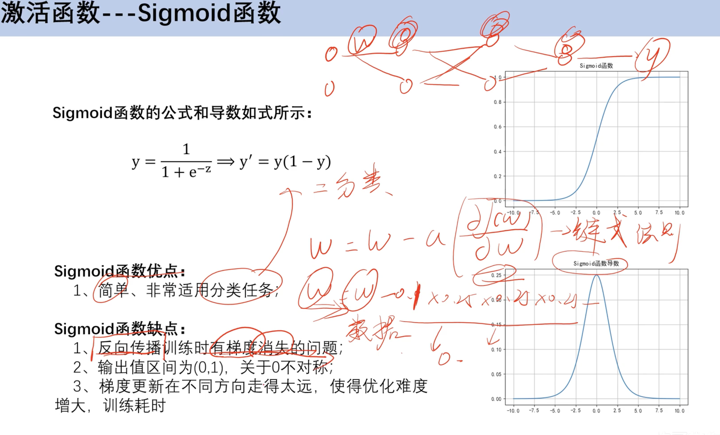
sigmoid函数
- 梯度消失问题,倒数图像左右消失太快 w
累计乘法后小数累成趋近于0
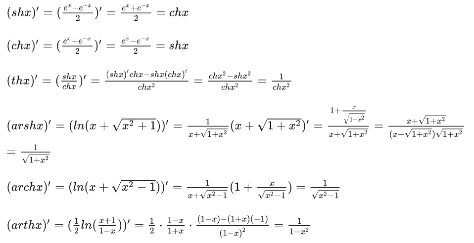
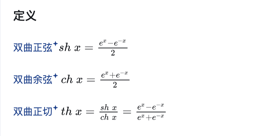
Tanh函数(双曲正切函数)
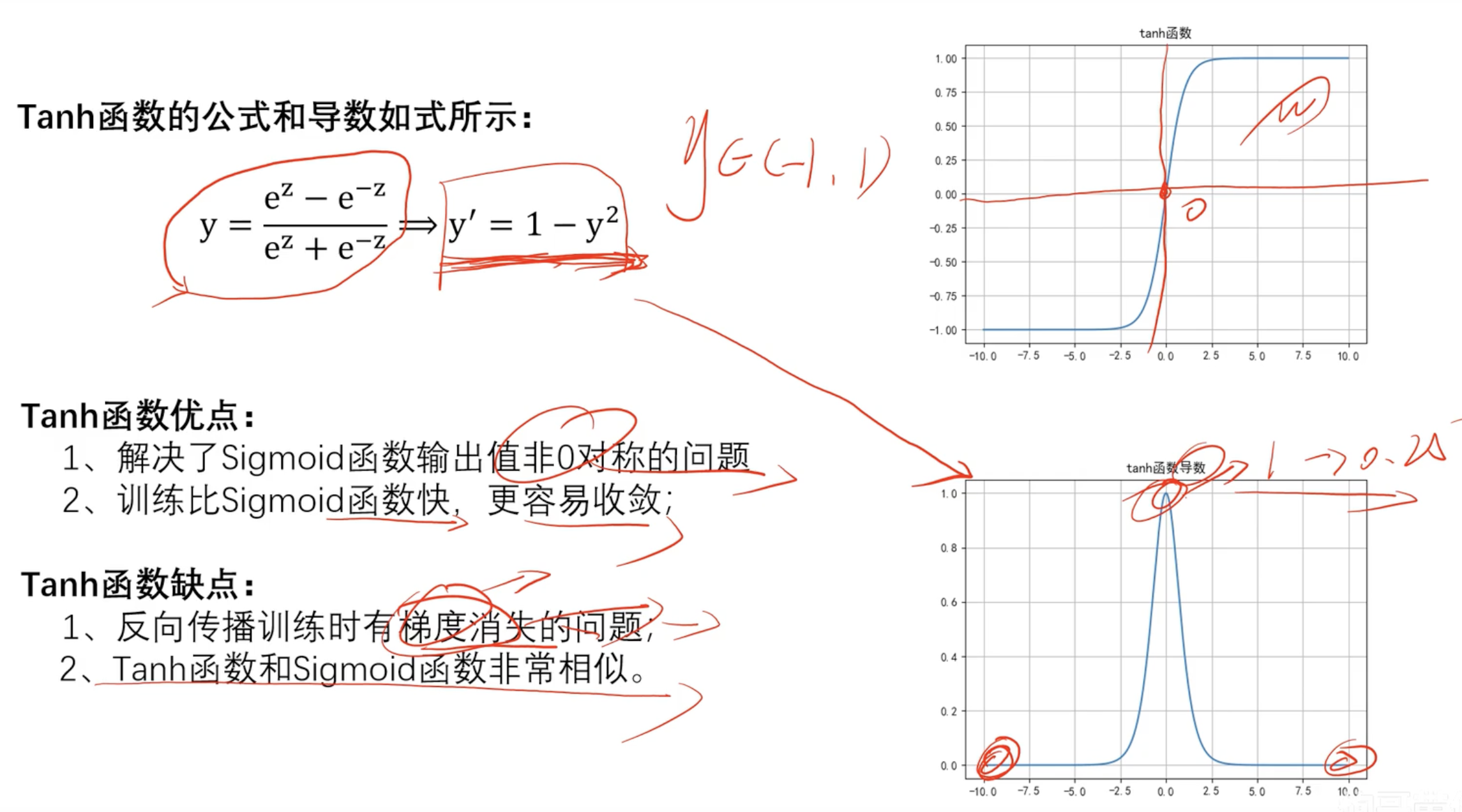
数学知识
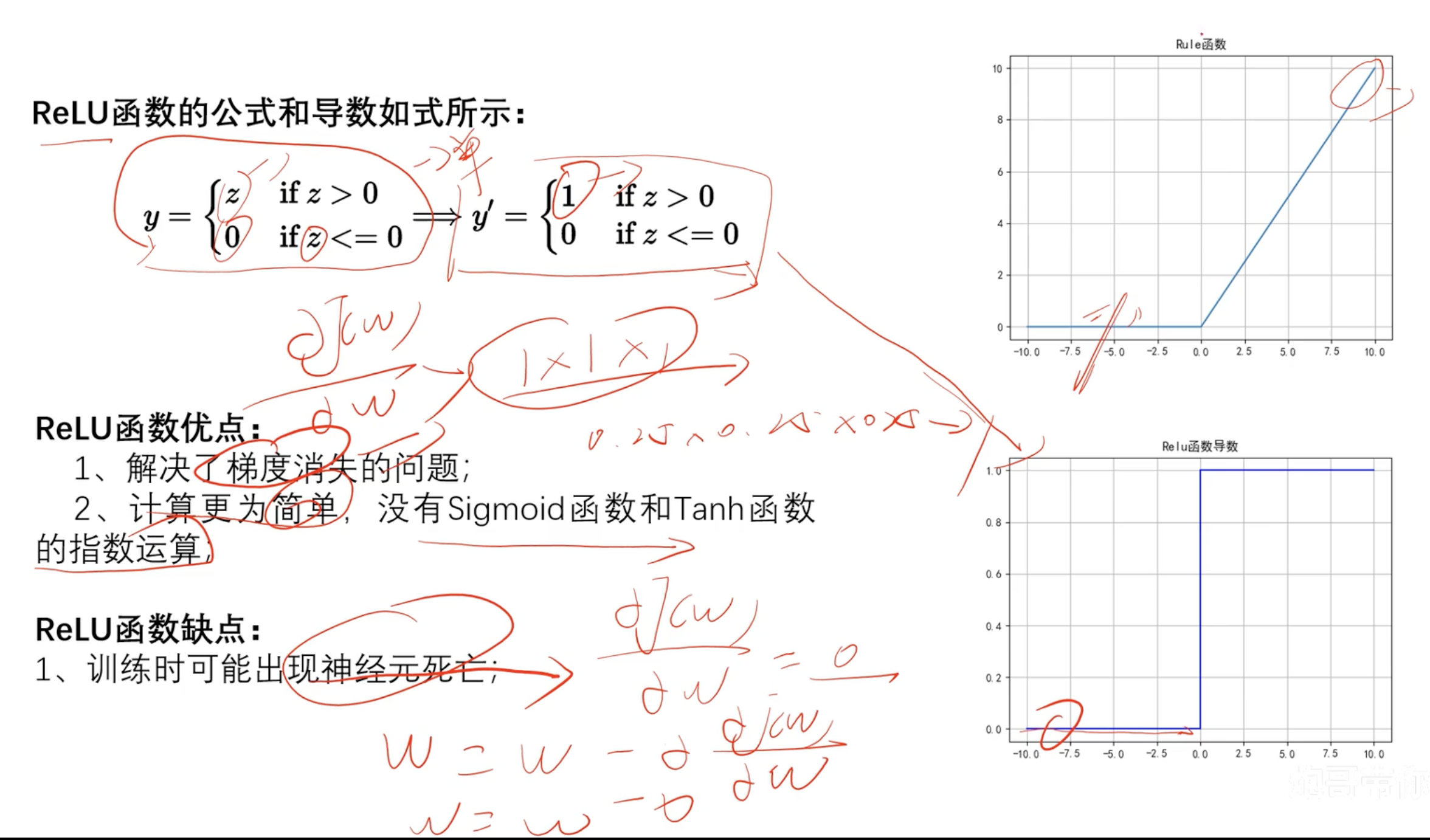
ReLU函数
- 神经元死亡:
z<0 倒数为0 w停止更新
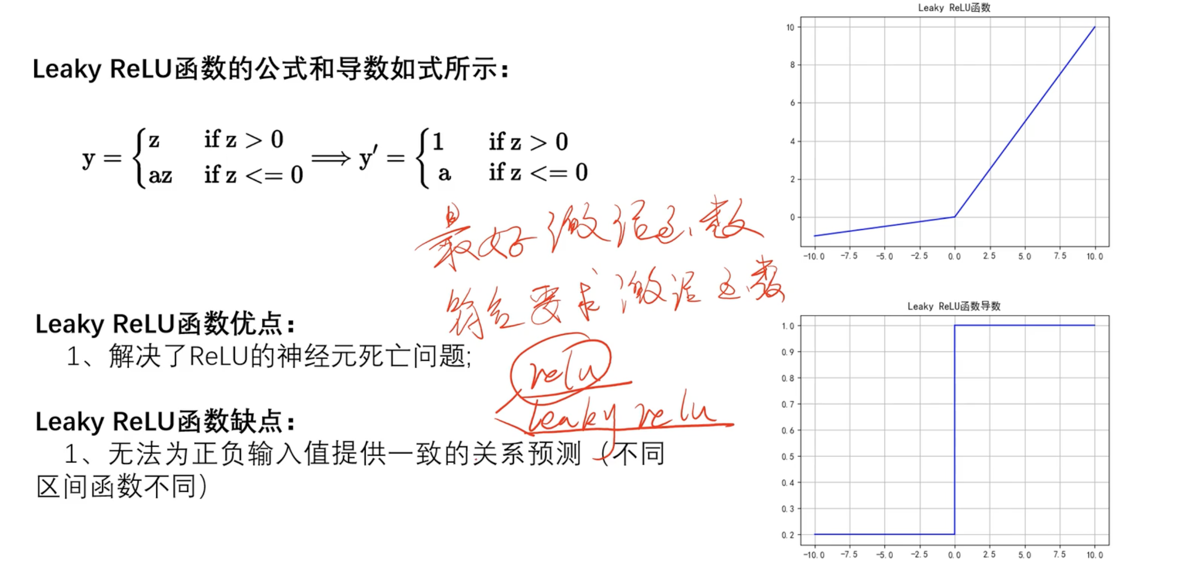
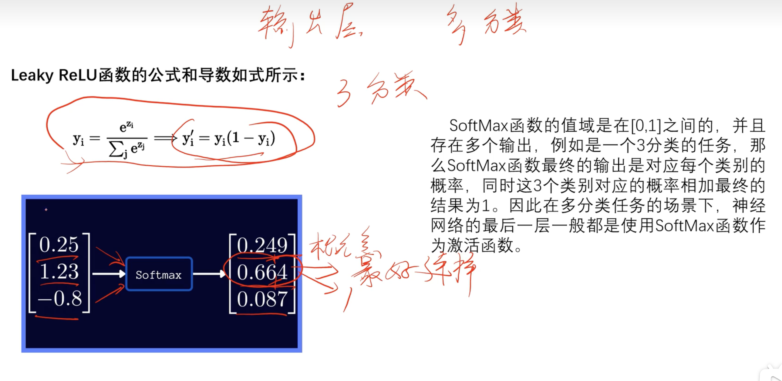
Leaky ReLU
- 没有最好的激活函数 只有符合的激活函数
SoftMax
用于多分类任务用于输出层
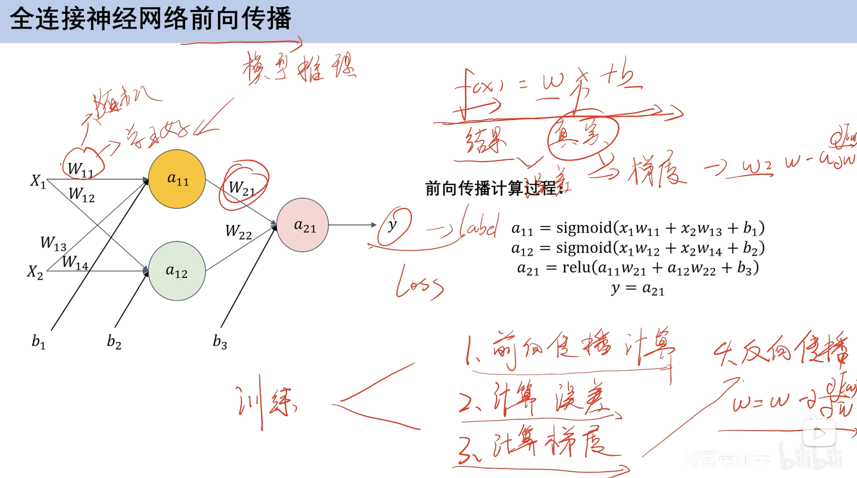
前向传播
前向传播计算预设w和b 根据数据集计算计算误差类比损失函数计算梯度梯度更新 求损失函数偏导反向传播反向更新w和b
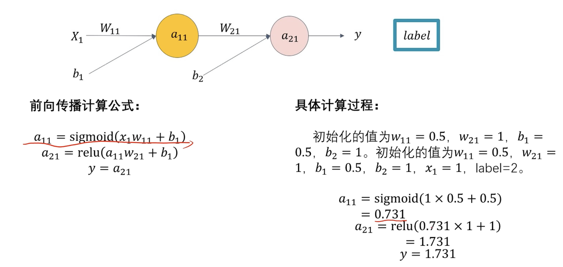
具体过程
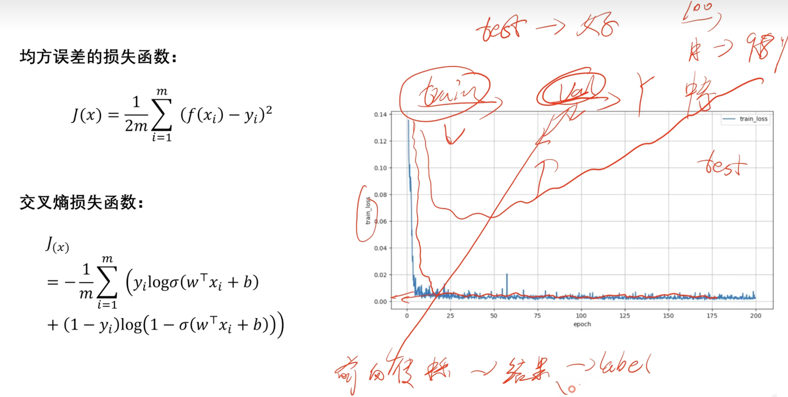
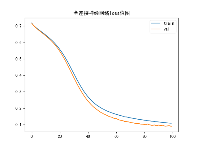
损失函数
图像解释:前面cost值逐渐减小,w,b逐渐吻合,前向传播过程,用的train训练集
后面趋近于0 可能是测试集test
链式法则(数学补充)
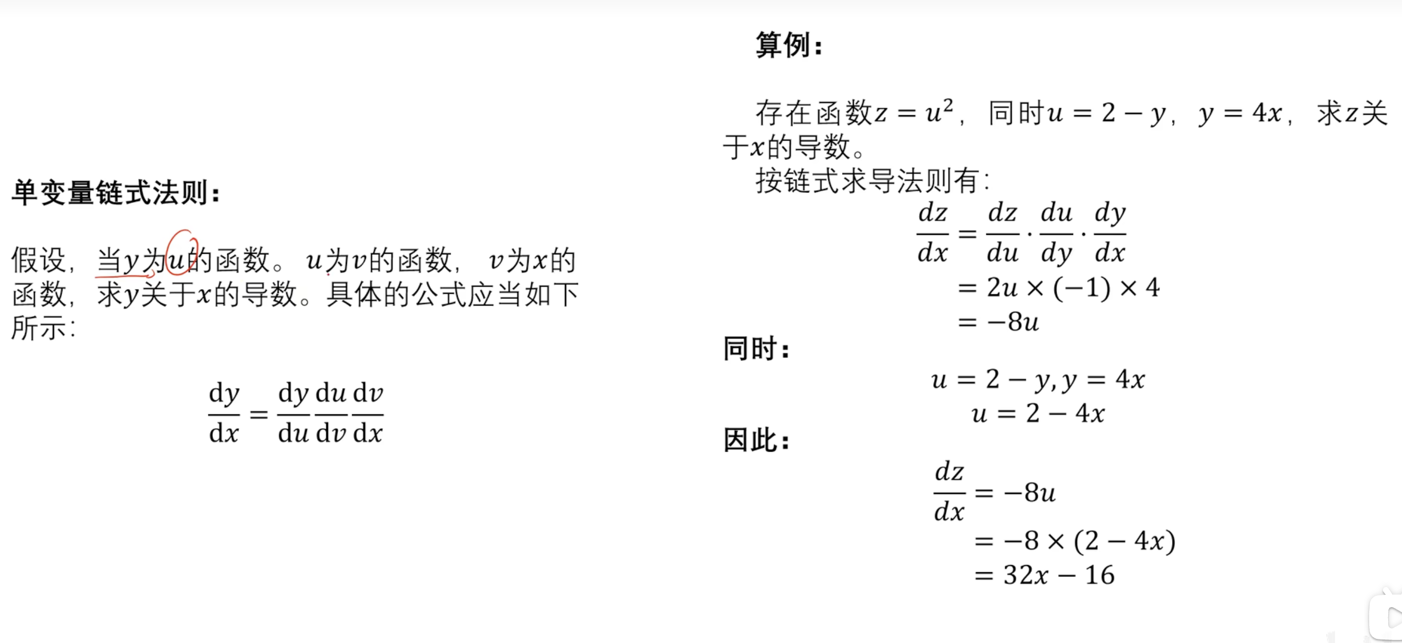
单变量链式法则
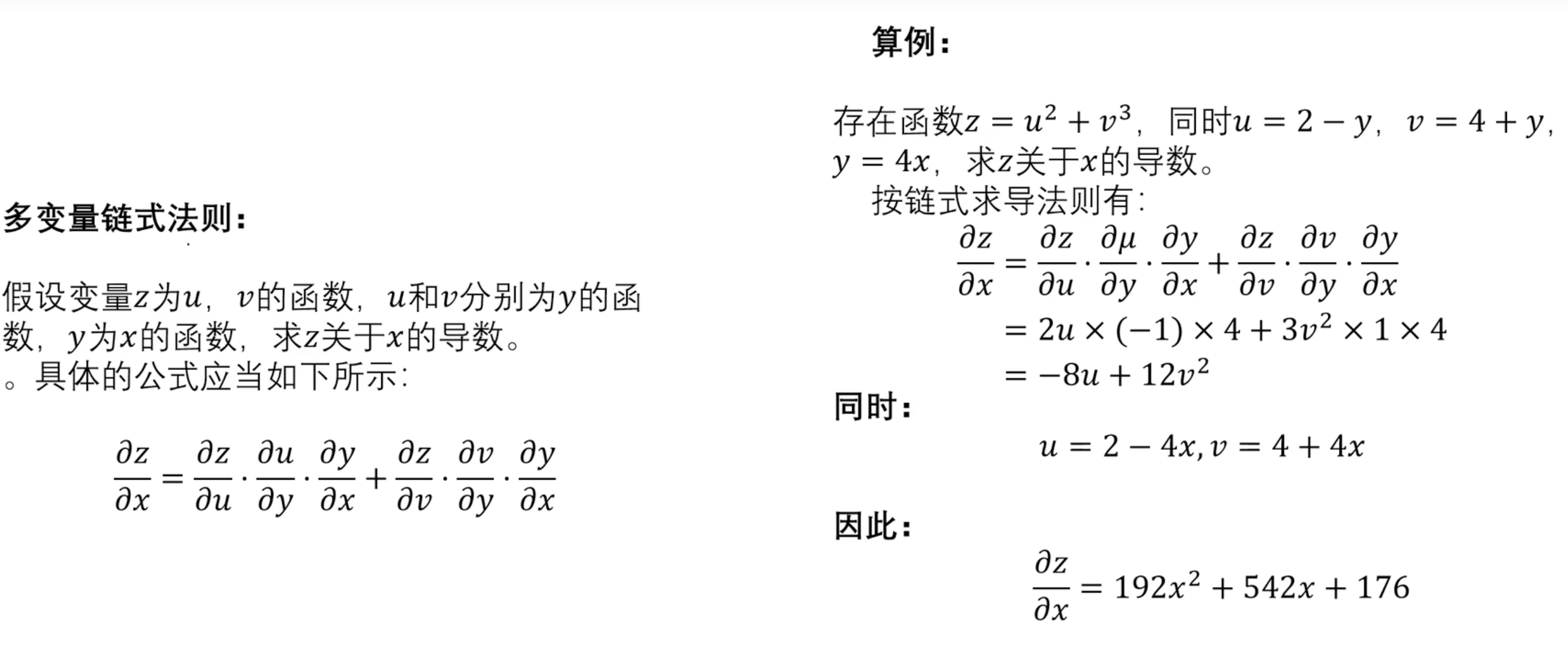
多变量链式发展
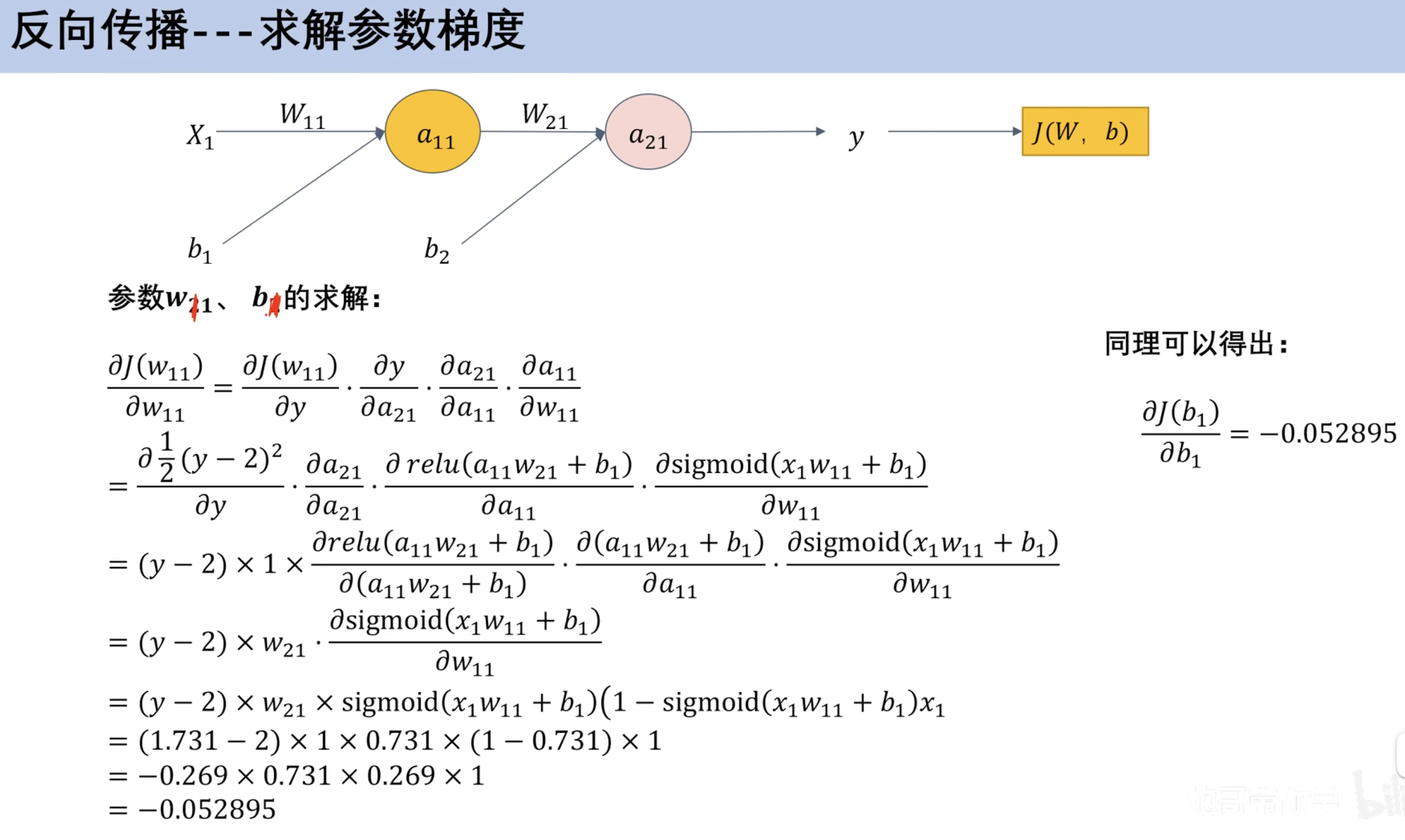
==反向传播==
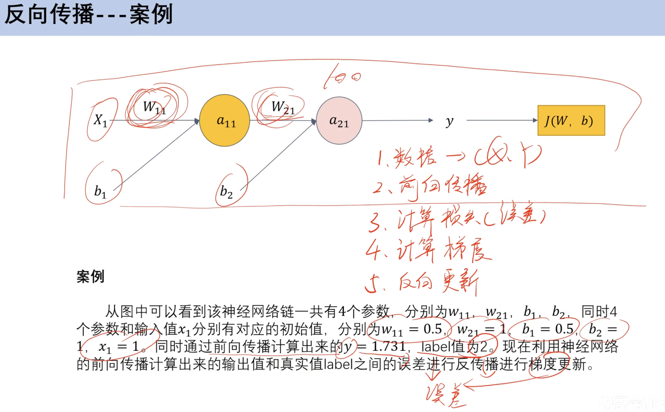
案例
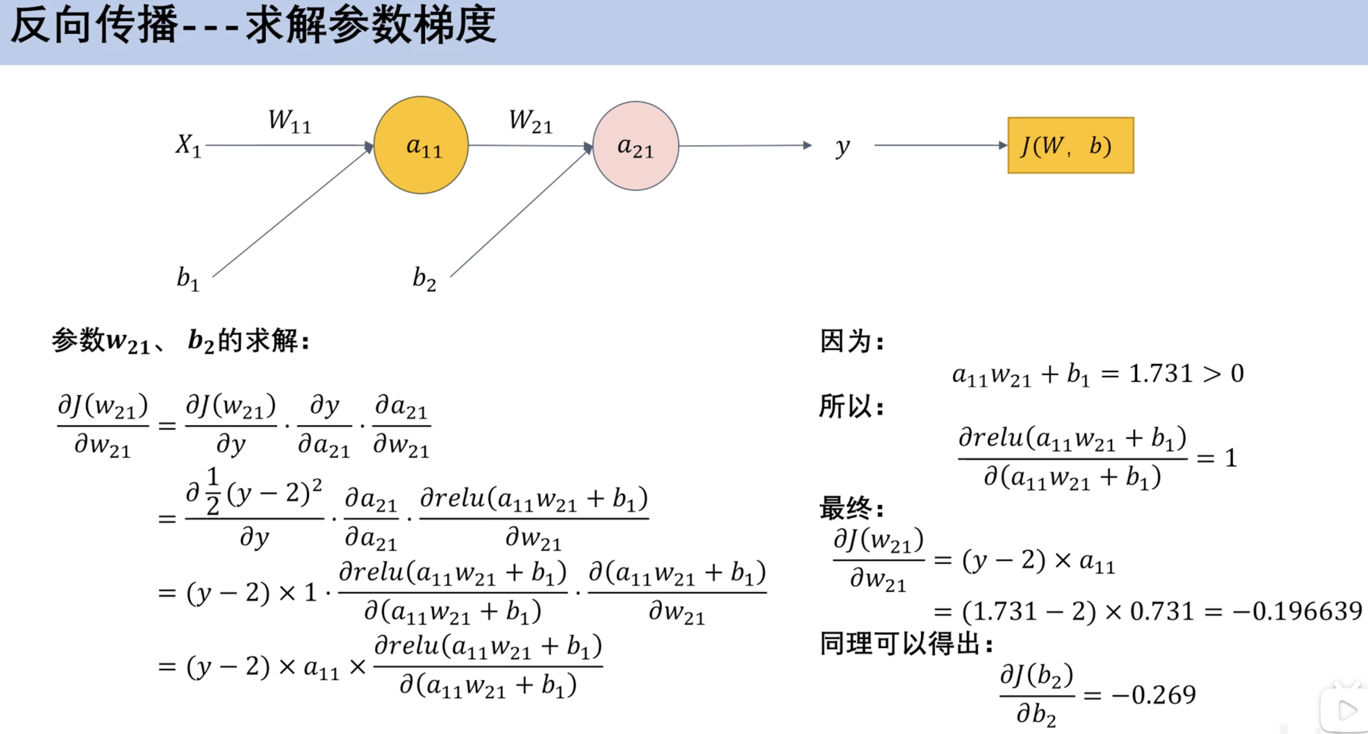
求解参数梯度
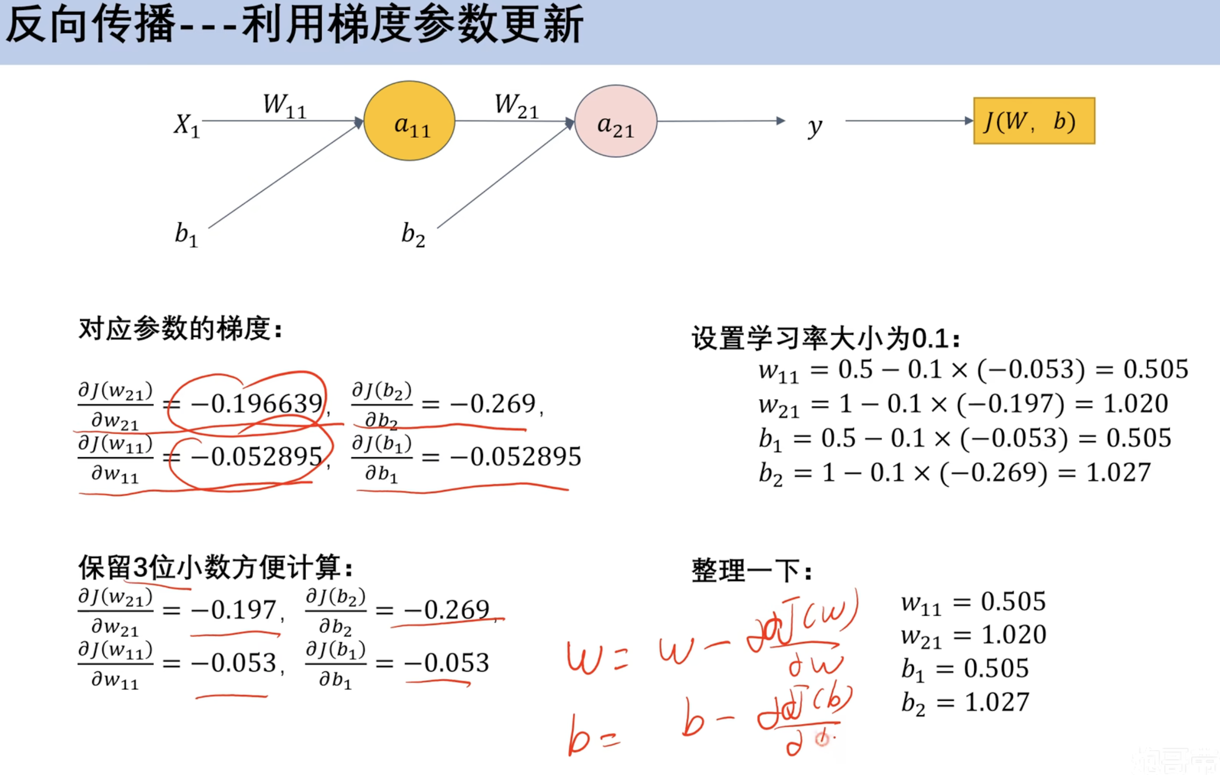
利用梯度参数更新
- 设置学习率为0.1
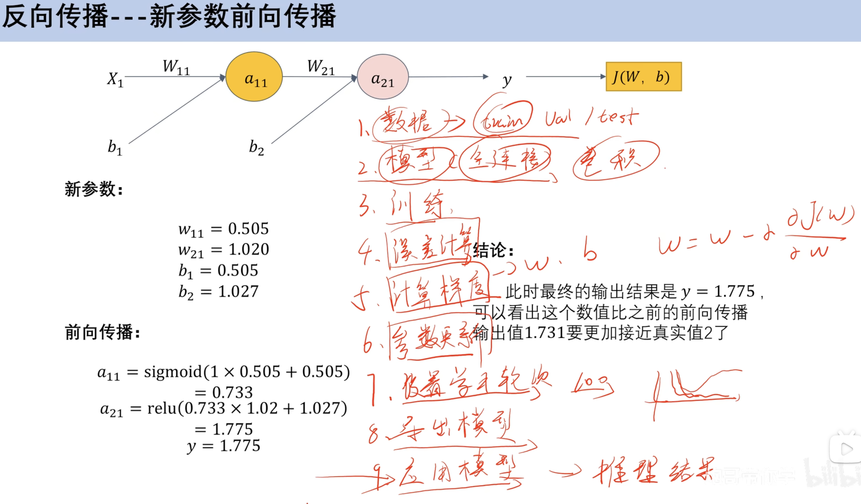
新参数前向传播
案例(预测乳腺癌 分类)
- 用全连接神经网络预测乳腺癌
- 对比机器学习
model_train
1 | import numpy as np |
model_test
1 | from cProfile import label |
函数图像
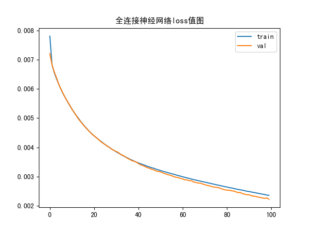
loss
accuracy
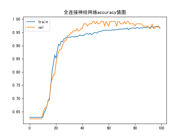
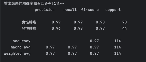
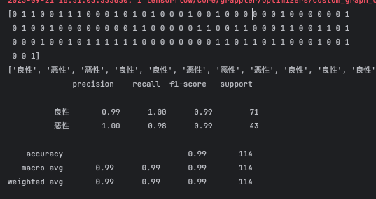
预测报告
案例(空气质量 线性回归)
model_train
1 | import numpy as np |
model_test
1 | import numpy as np |
loss图像
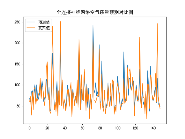
真实值预测值对比图
卷积神经网络CNN
计算机图片本质(引入)
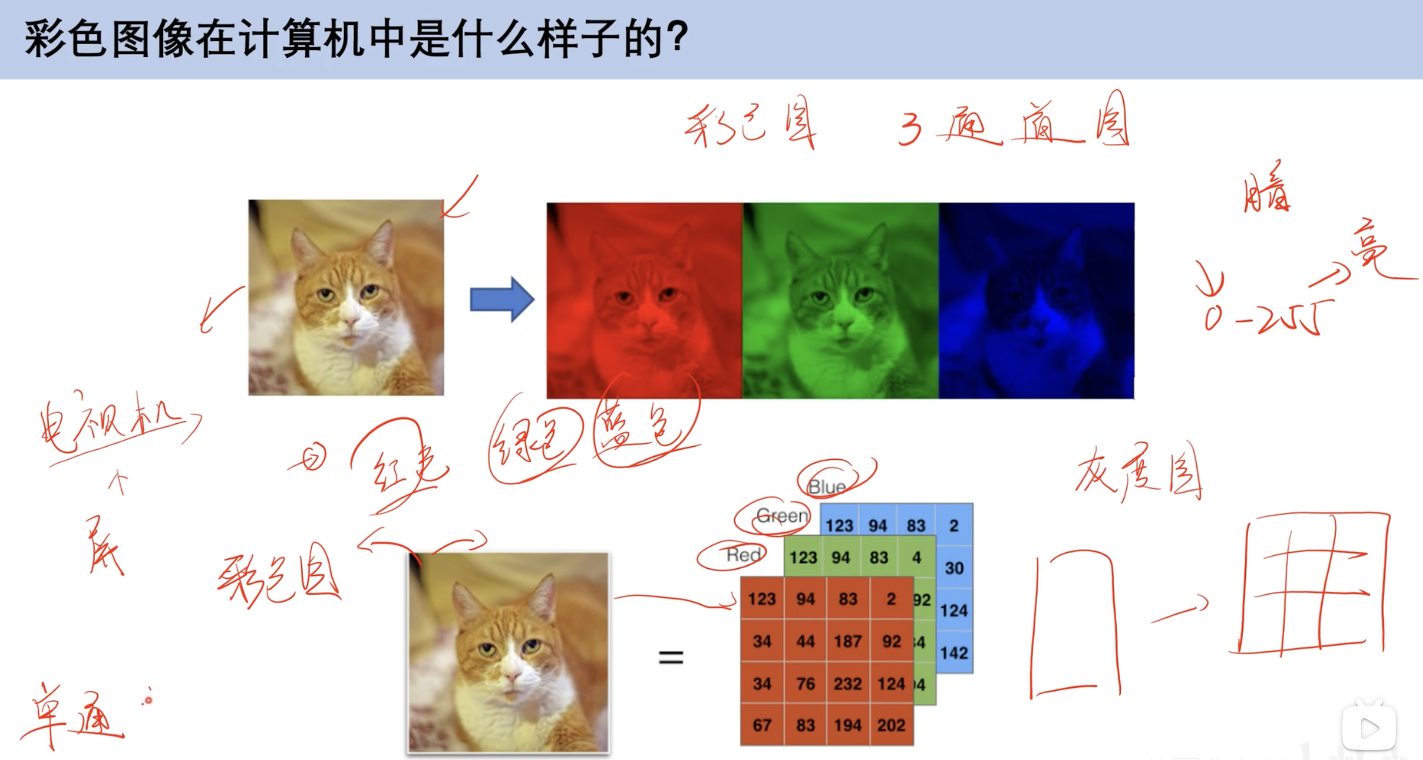
整体结构
- 卷积层:可以改变层数
- 池化层:可以改变高度

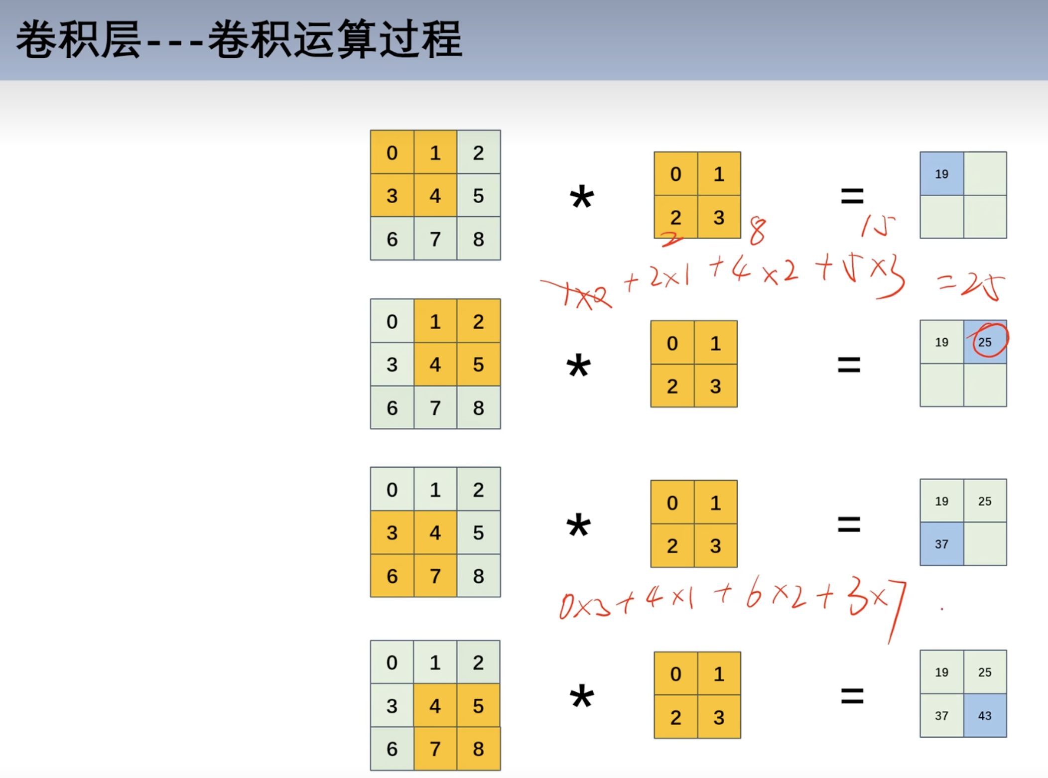
卷积运算和权重共享
- 对应位置相乘
- 如第一行:
0*0 + 1 * 1+ 3*2+3*4
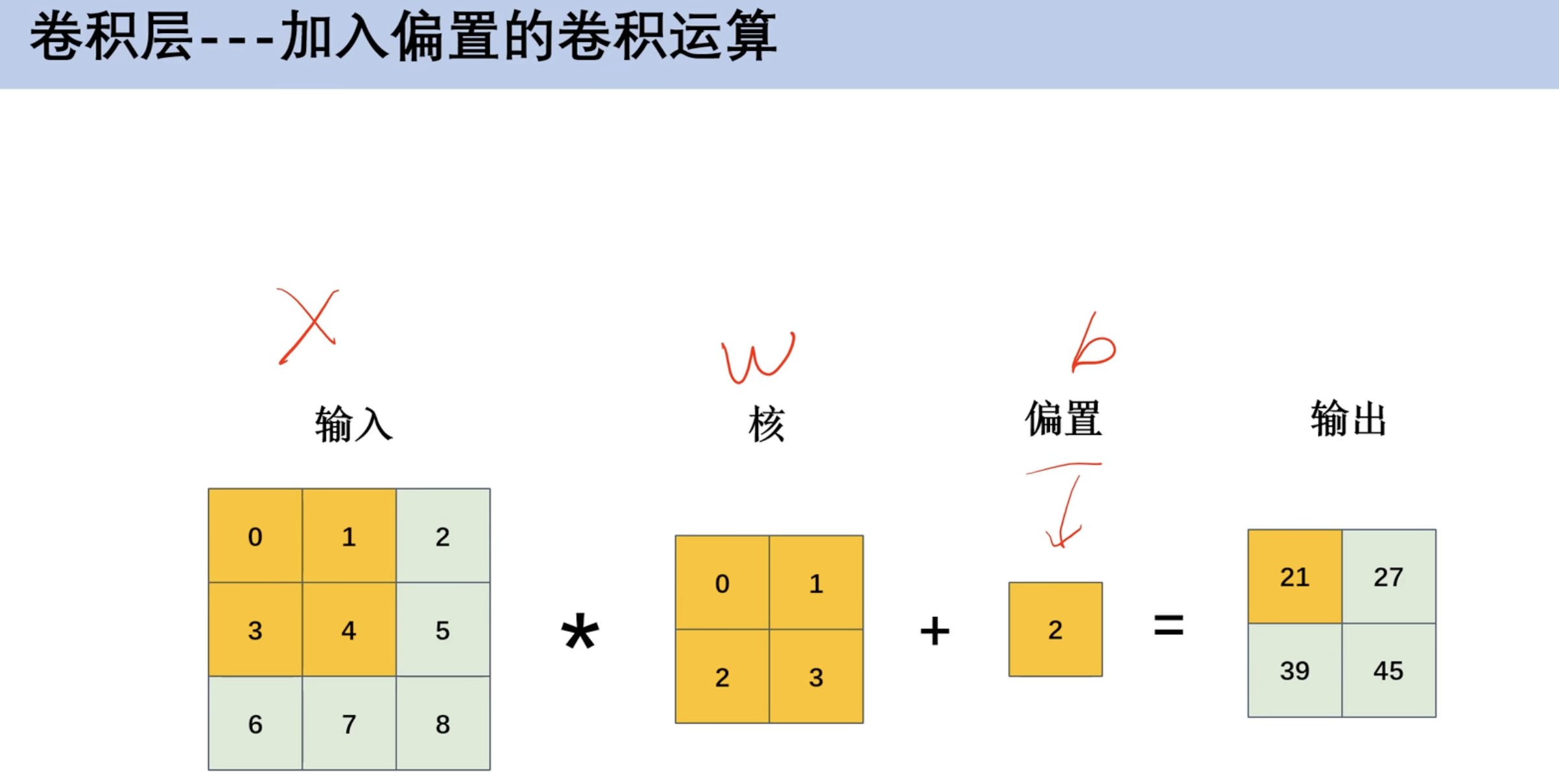
- 加入偏置
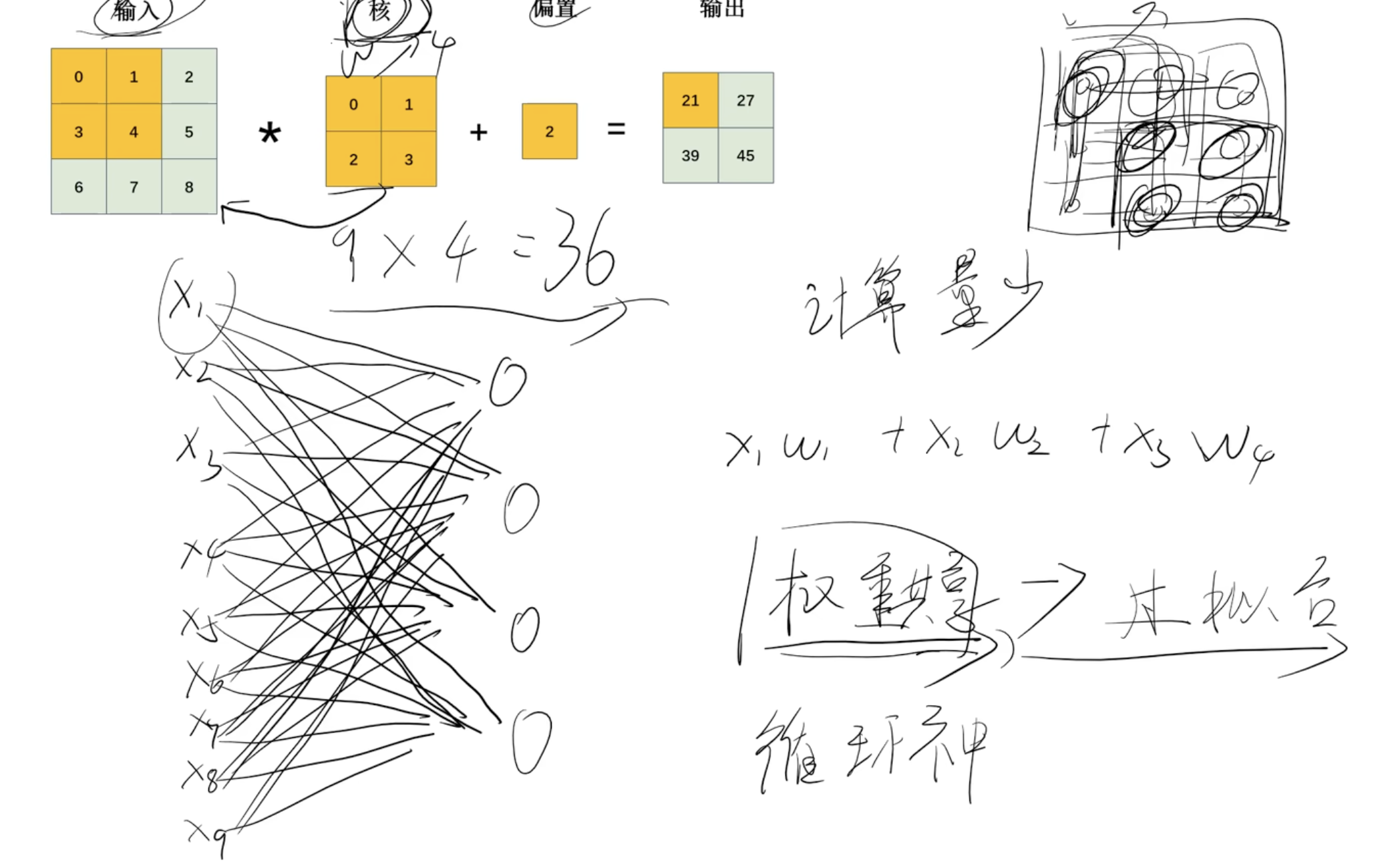
- ==权重共享==
- 矩阵中的数字有重叠w的情况
- 九个数据在全连接神经网络有36个w,在卷积神经网络有4个w,有效解决过拟合问题
- 在循环神经网络RNN也设计权重共享
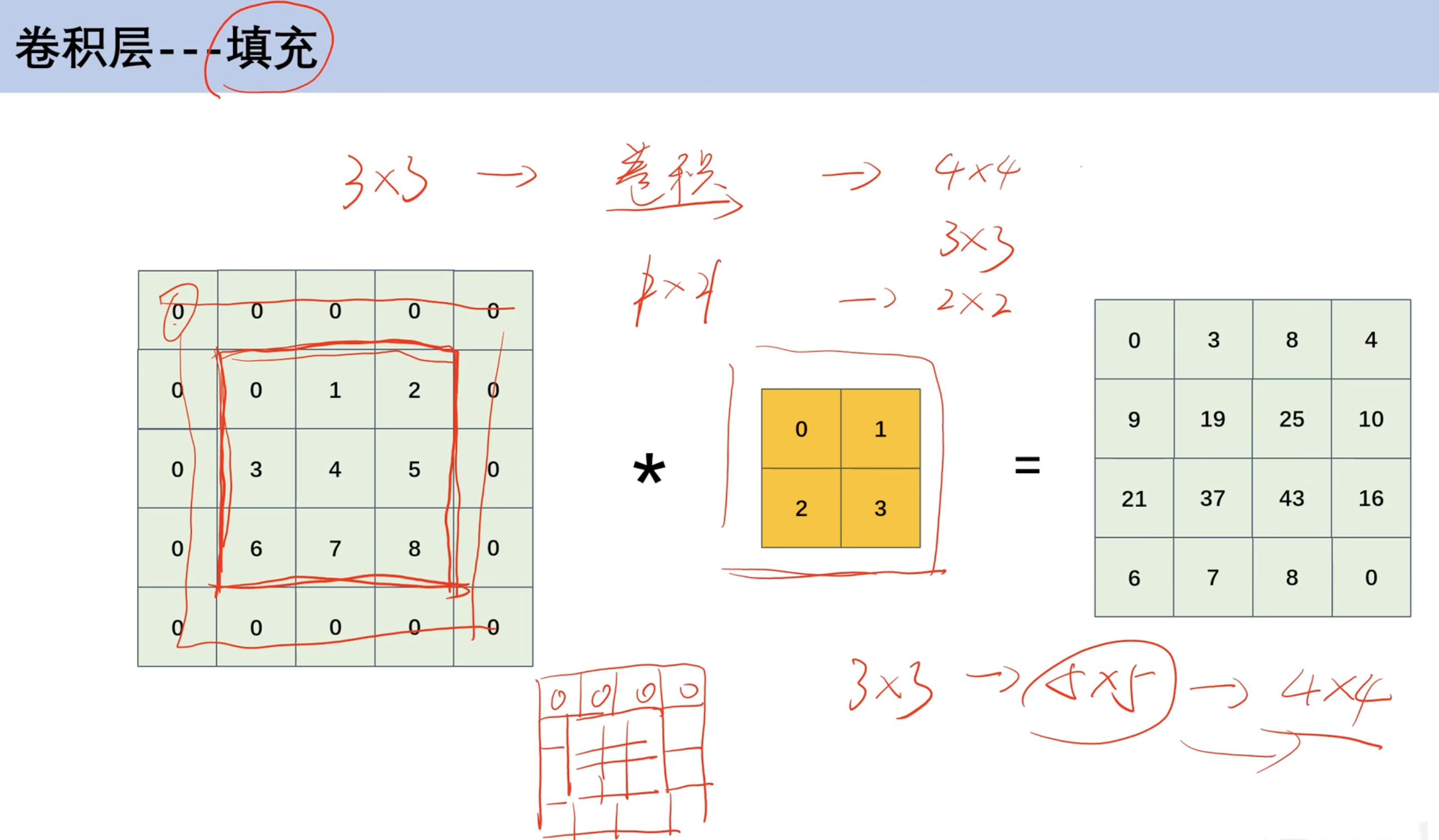
填充运算和步幅运算
- 填充运算
- 原本矩阵
3*3- 在外面一层扩充0像素
5*5- 对
5*5像素做乘法得到4*4
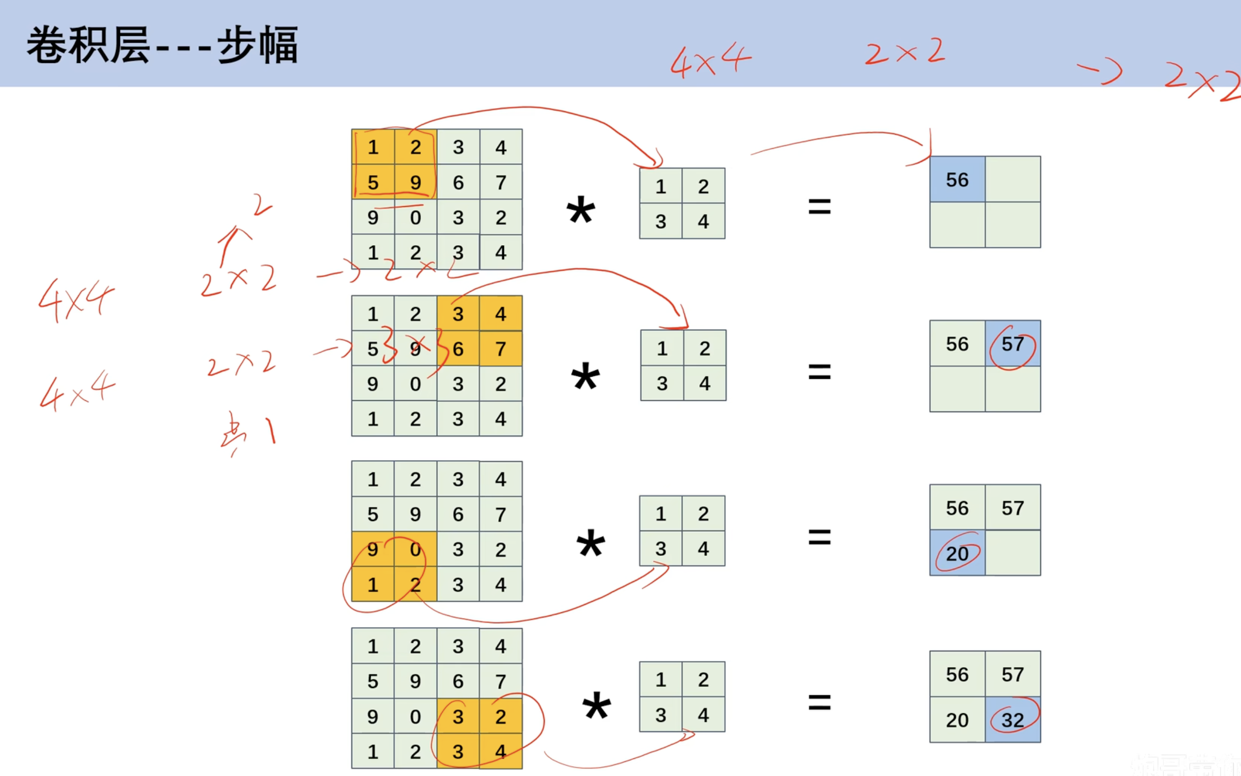
- 步幅
- 上面的计算默认步幅为1
- 可以调整步幅,如此时调整为2
4*4*2*2得到2*2(步幅为2)
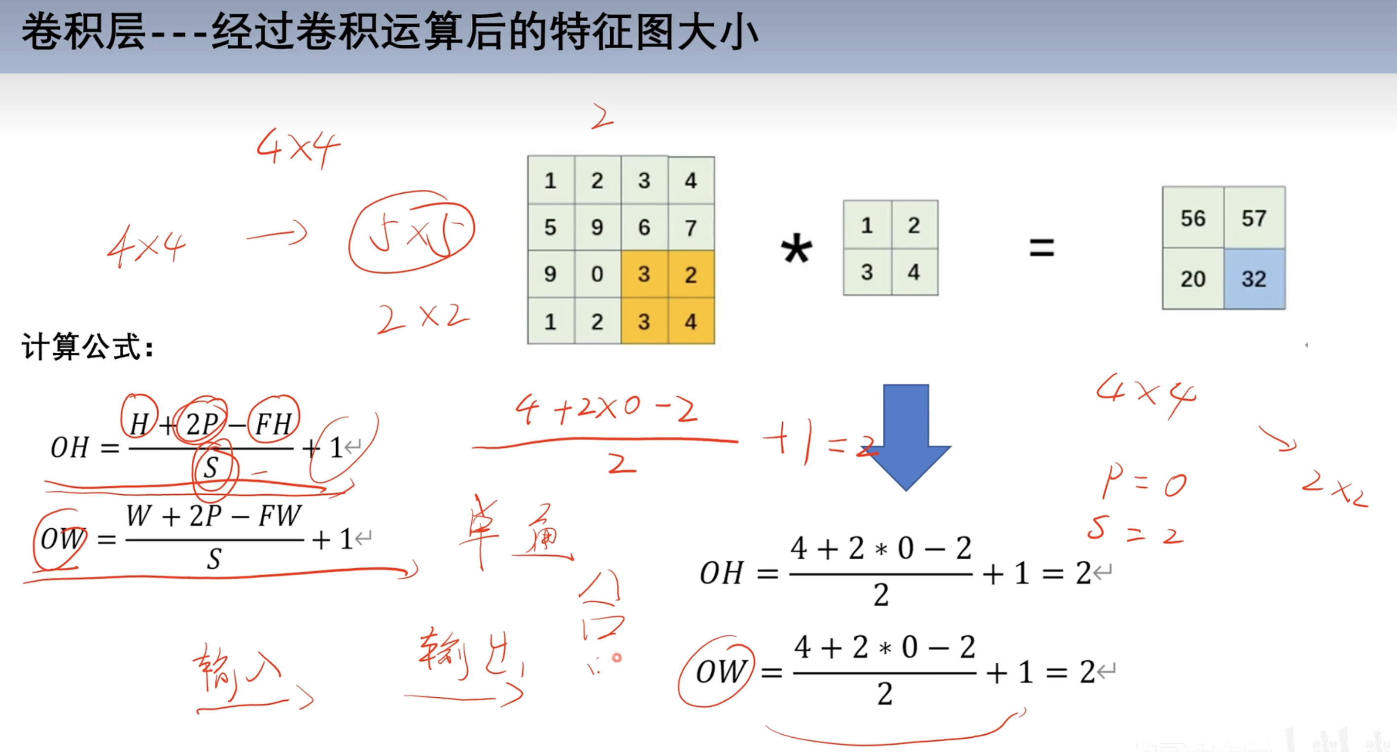
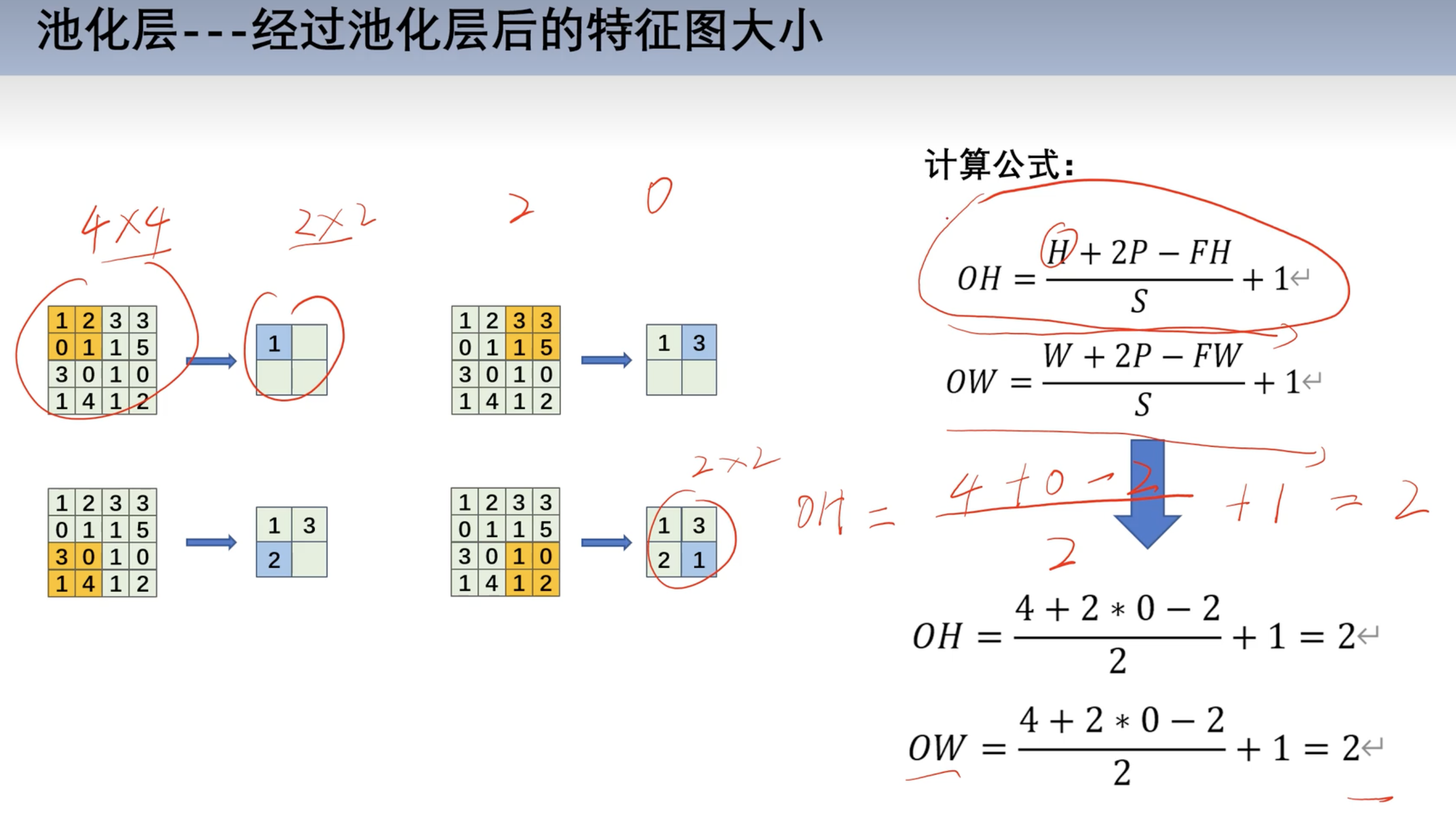
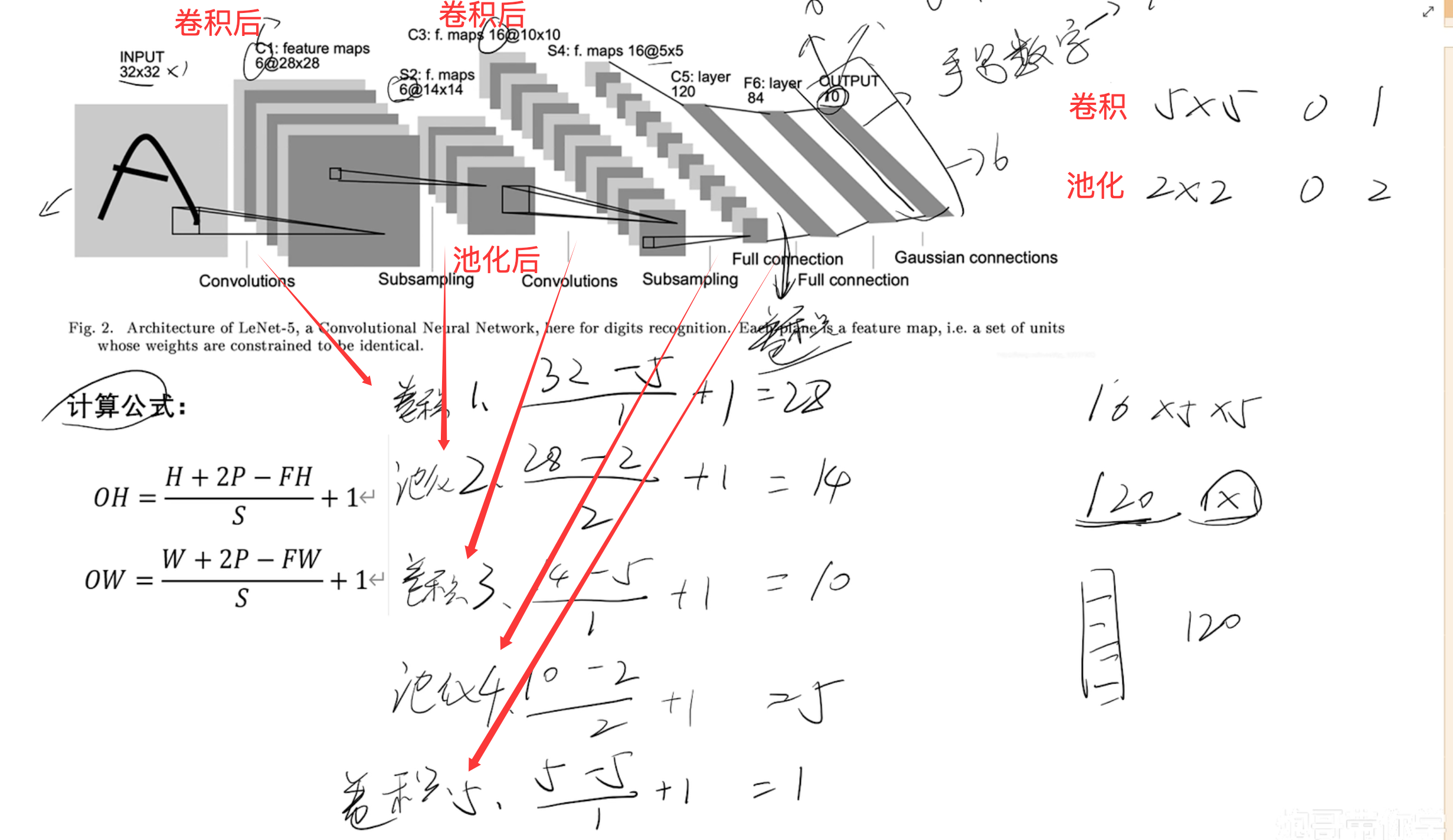
- 公式
- H 高
- P 填充高度
- FH 核的高度
- S 步幅
- OH 输出高度
- OW 输出宽度
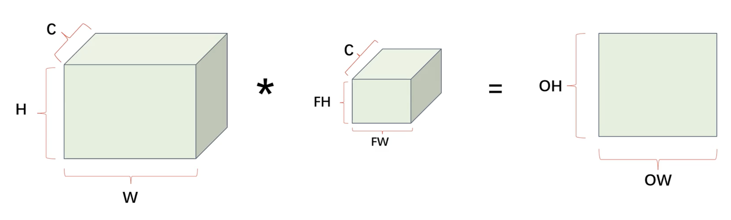
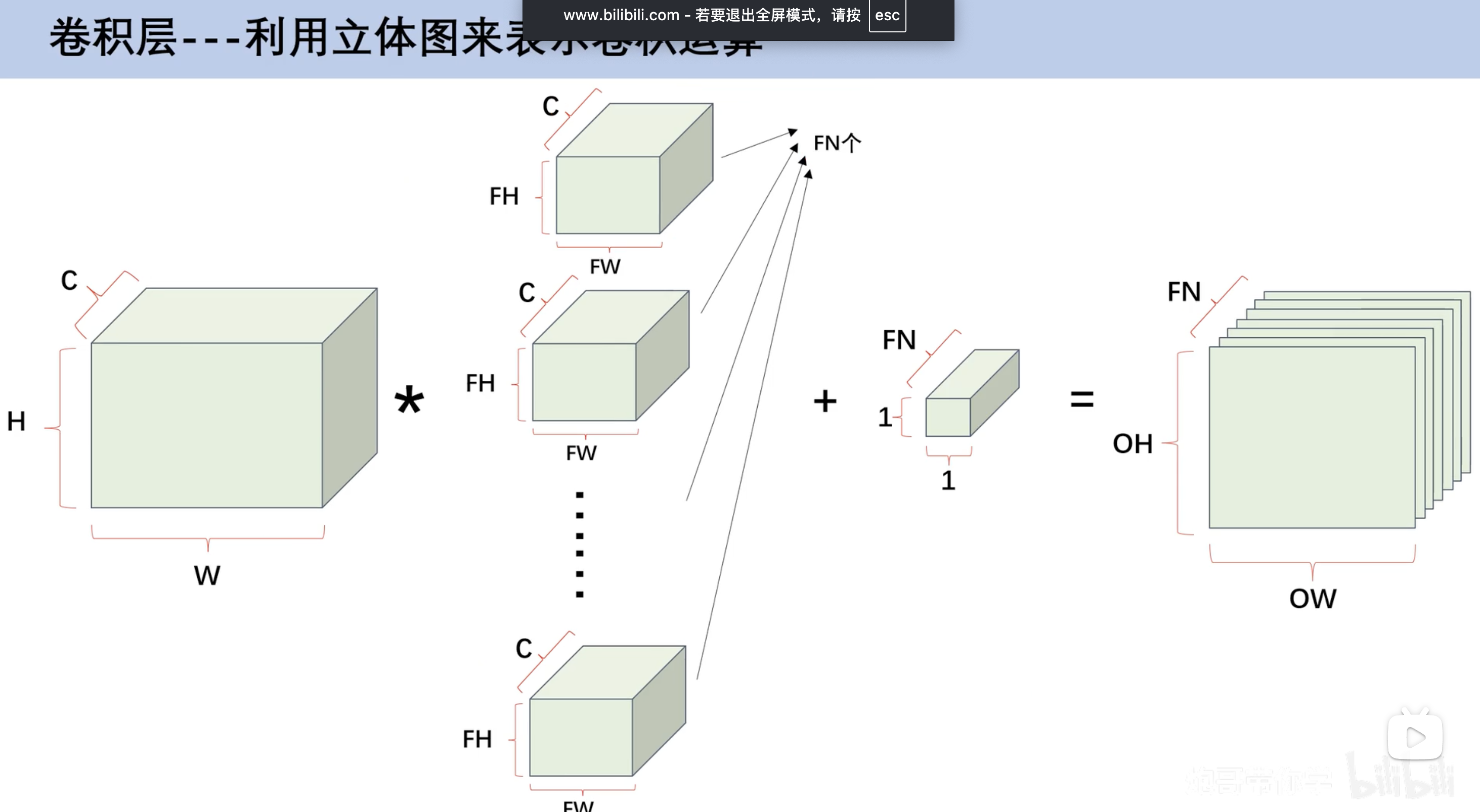
多通道卷积运算
- 对应的卷积相乘
- 再相加
- 通道数(特征图数量)相同才能相乘
- 最后得到的结果都是一张特征图
- 若要得到n张特征图 需要n份核图
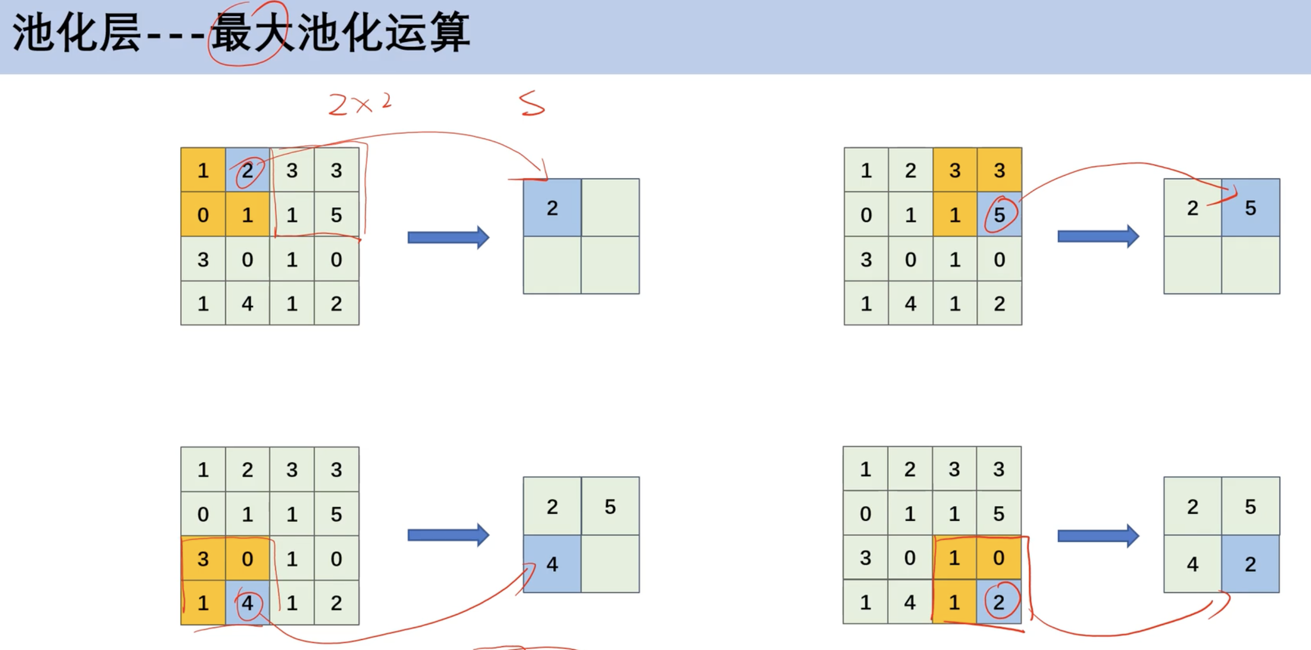
池化运算
最大池化
- 本质: 在每组中取特殊值
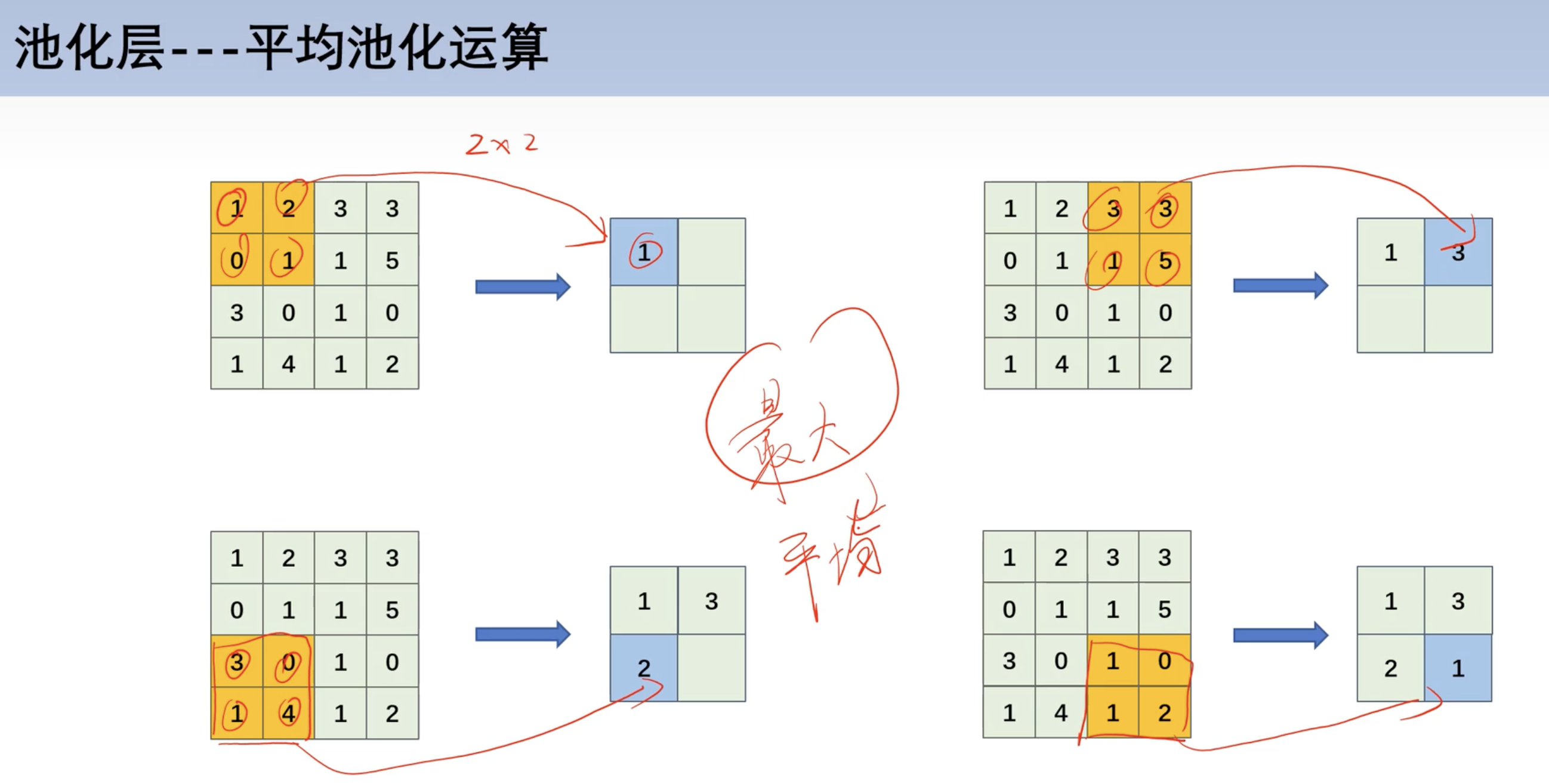
平均池化
- 一般来说,最大池化比平均池化用的多
池化公式
实战(LENET) 目标缺陷检测
maps6@28x286个特征图 每张图28*28
model_train
1 | import pathlib |
model_test
1 | import numpy as np |
循环神经网络
RNN
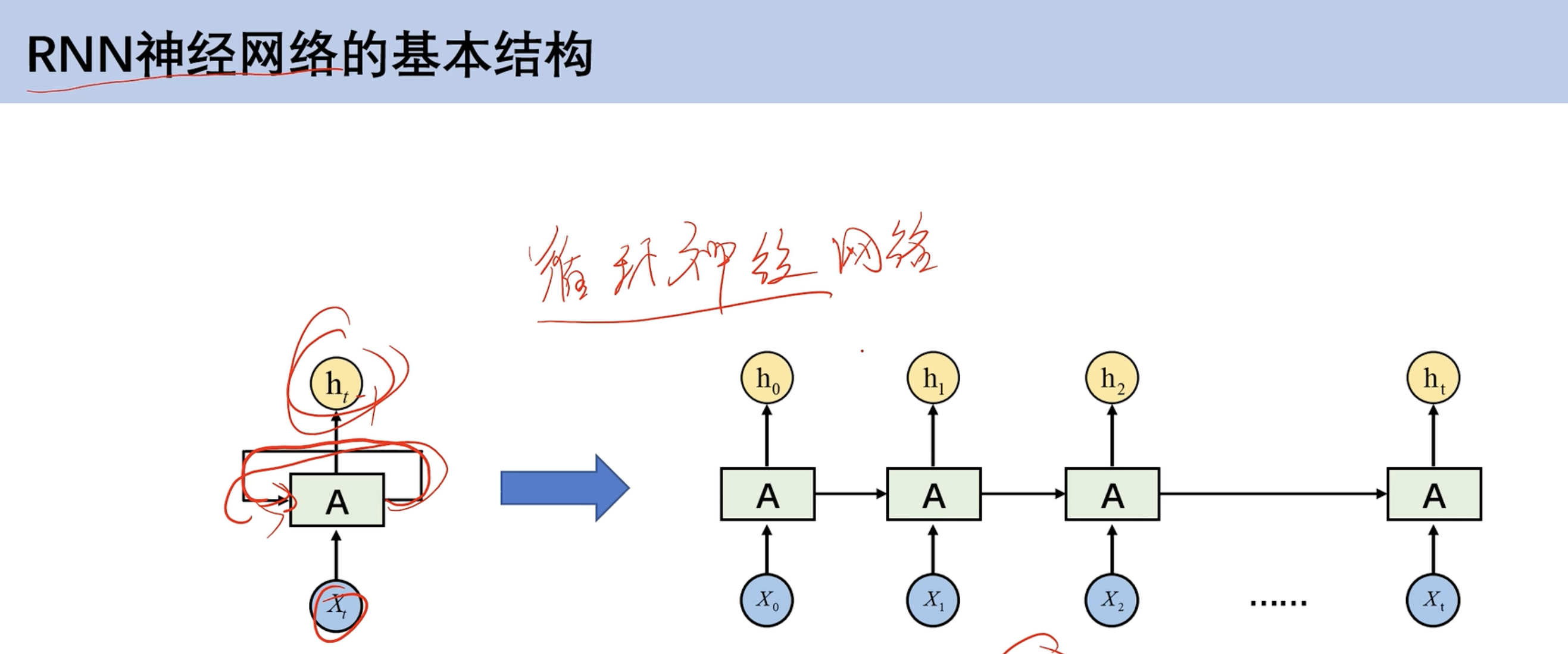
RNN基本结构
- h0不仅作为第一个隐藏层输出 也作为第二个隐藏层输入
- 先计算t0时刻,接着t1。有先后顺序
- CNN则是同时输入 只有空间维度
- RNN加入时间维度,受之前数据影响
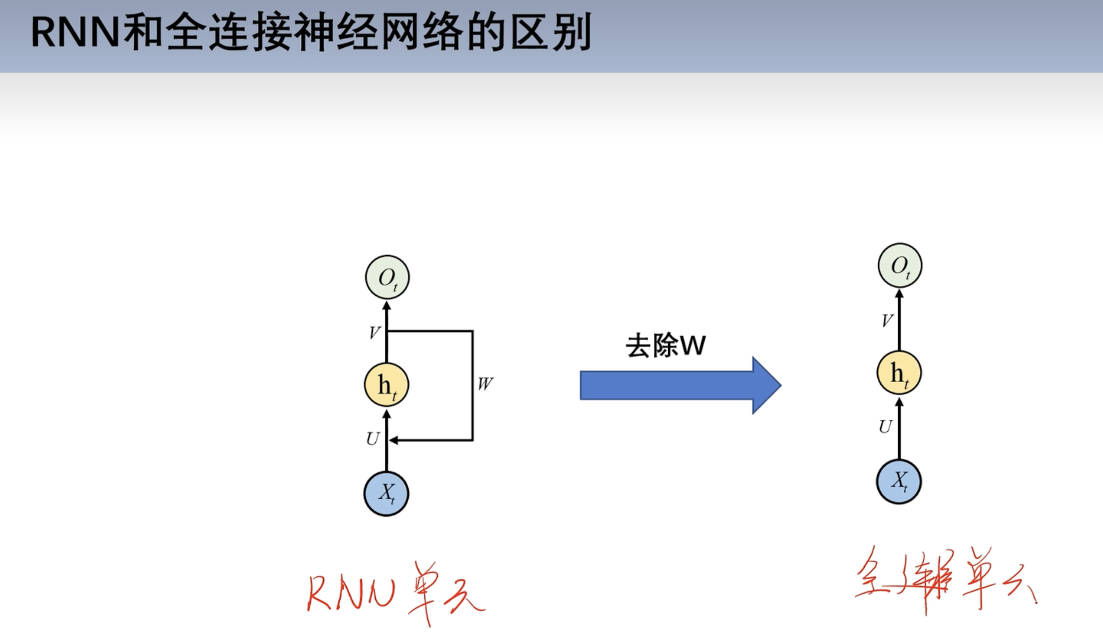
RNN和全连接神经网络区别
- 去掉W和全连接神经网络一样
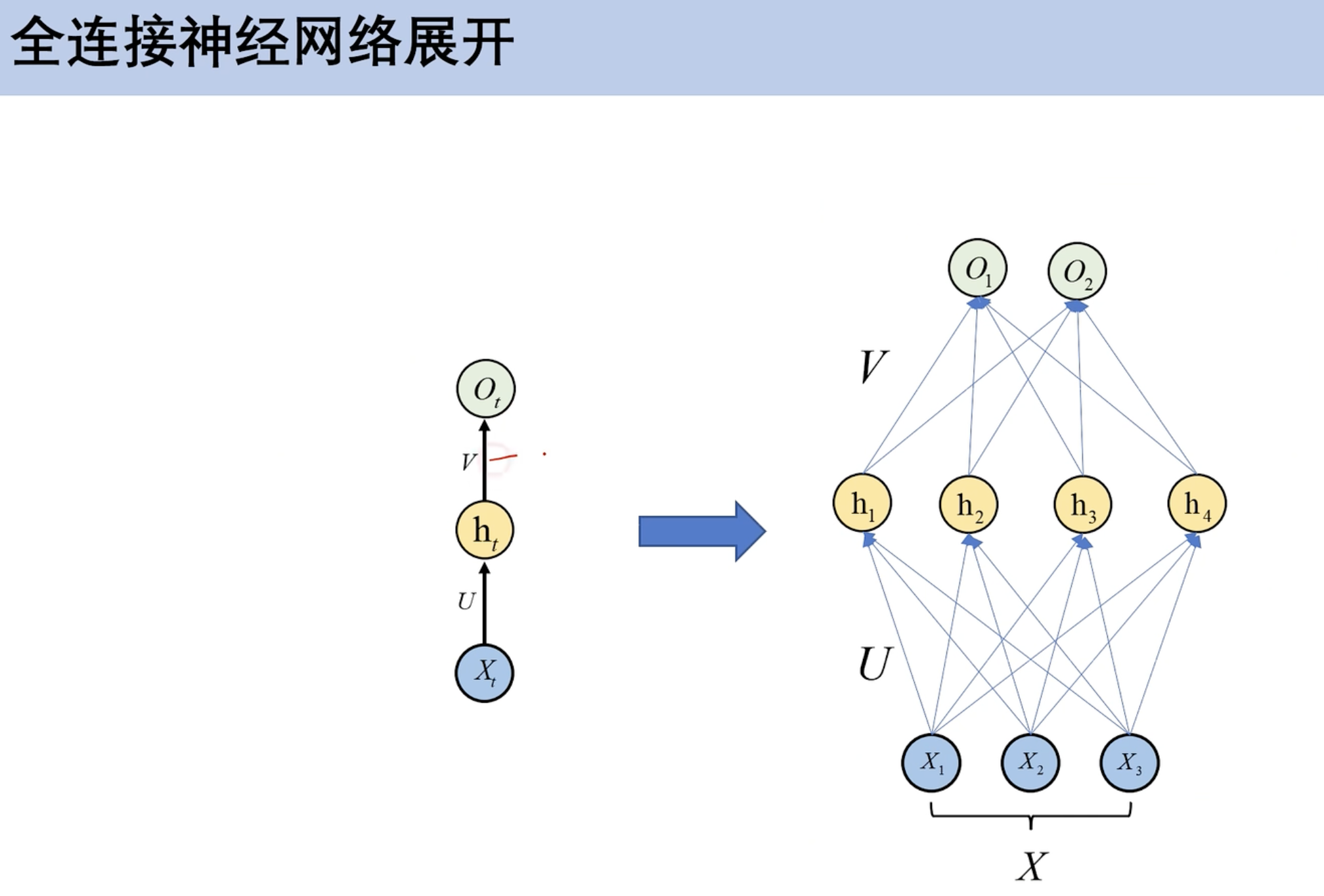
全连接展开
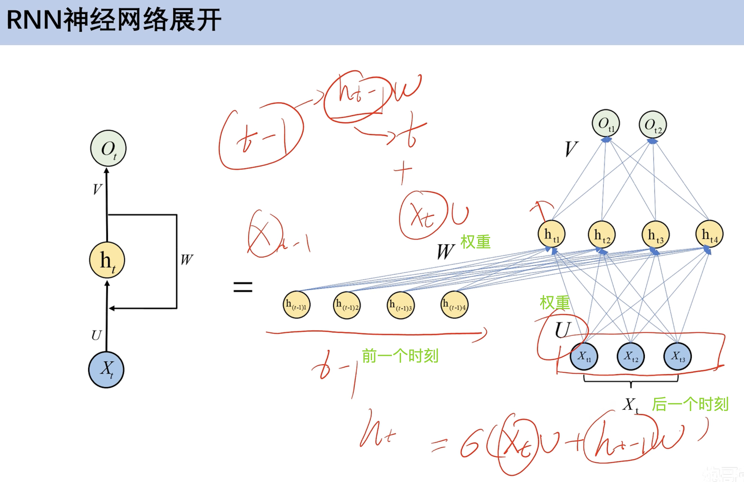
RNN展开
- 前一个时刻hw + 后面时刻hU
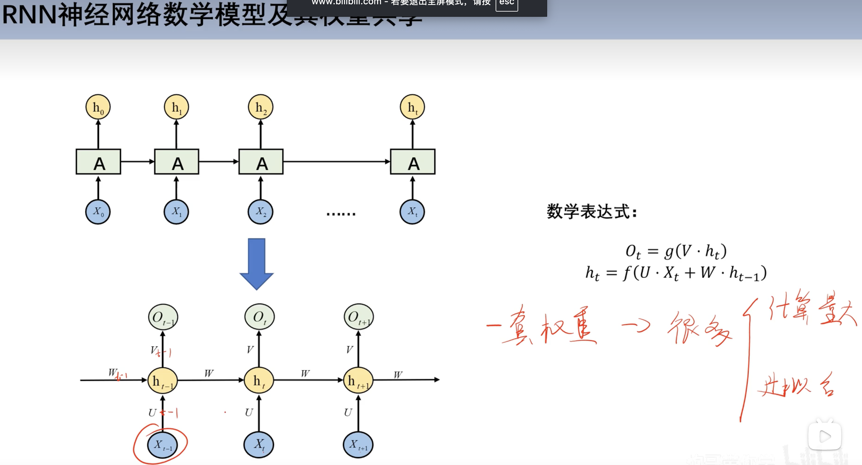
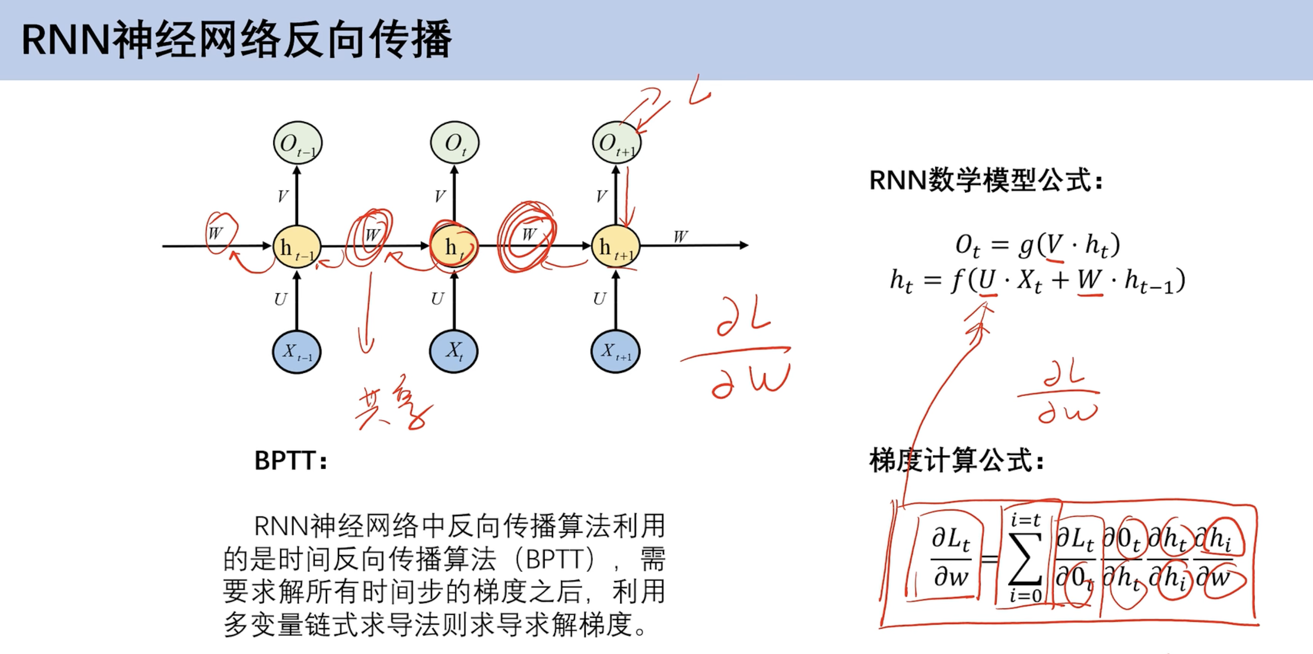
数学模型及权重共享
- 每个时刻对应的权重w和v相同
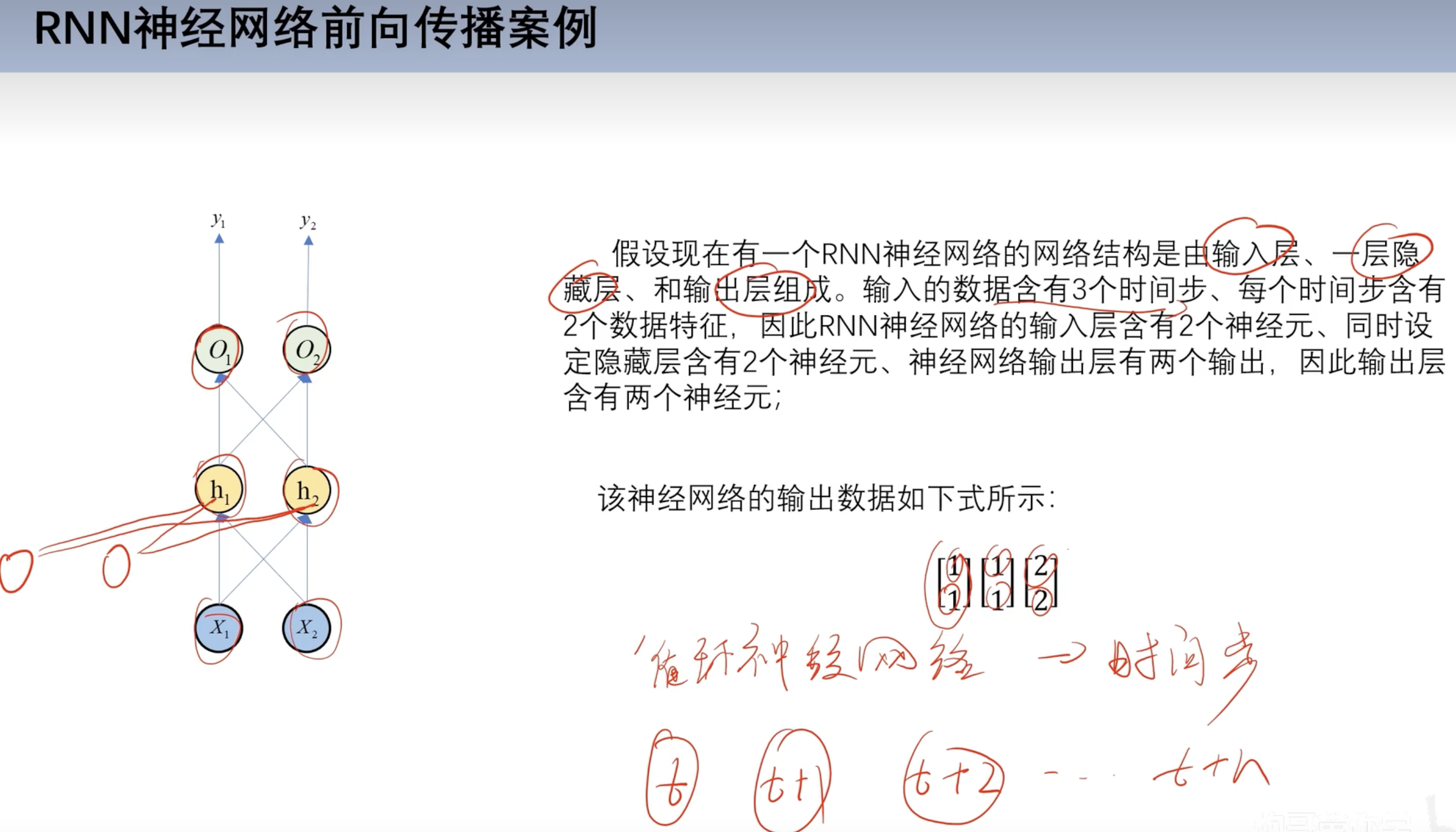
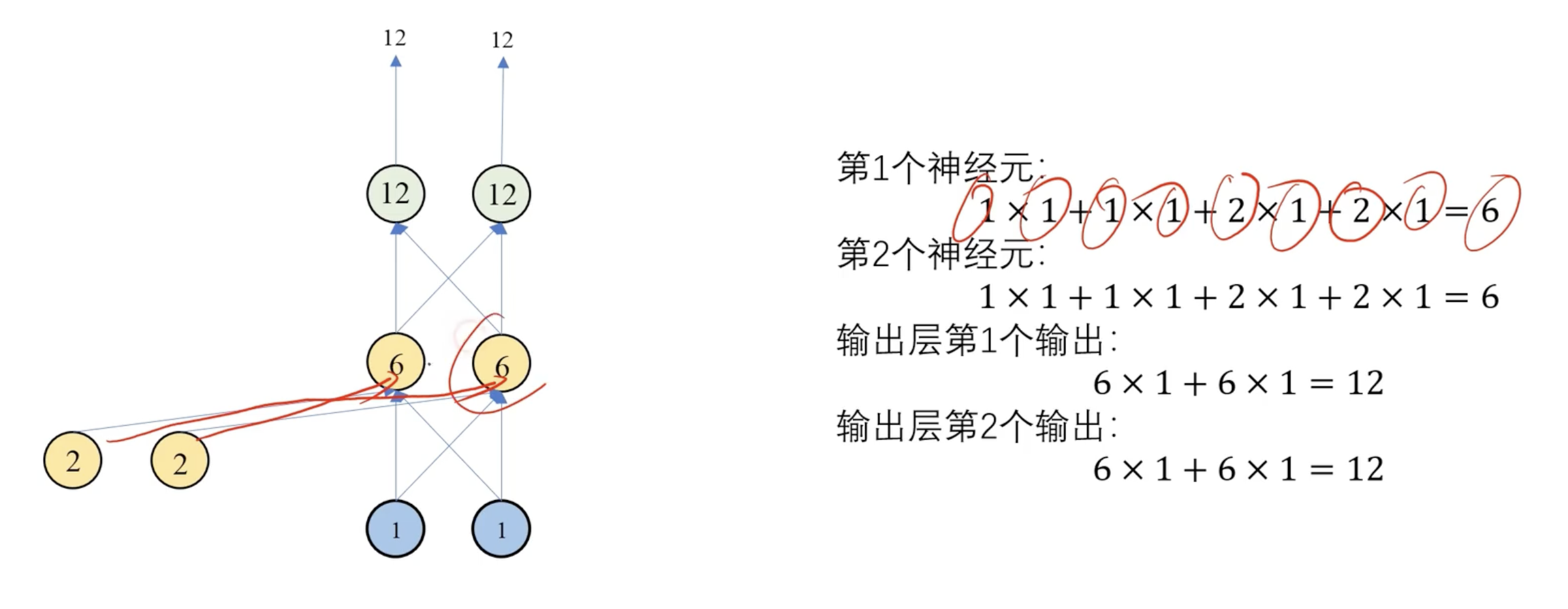
前向传播案例
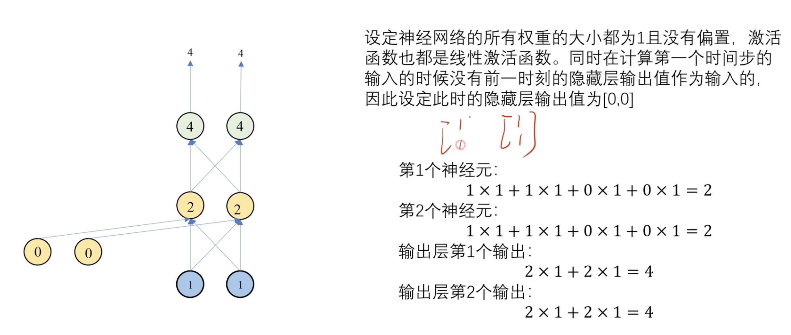
第一个时间步
第二个时间步
反向传播
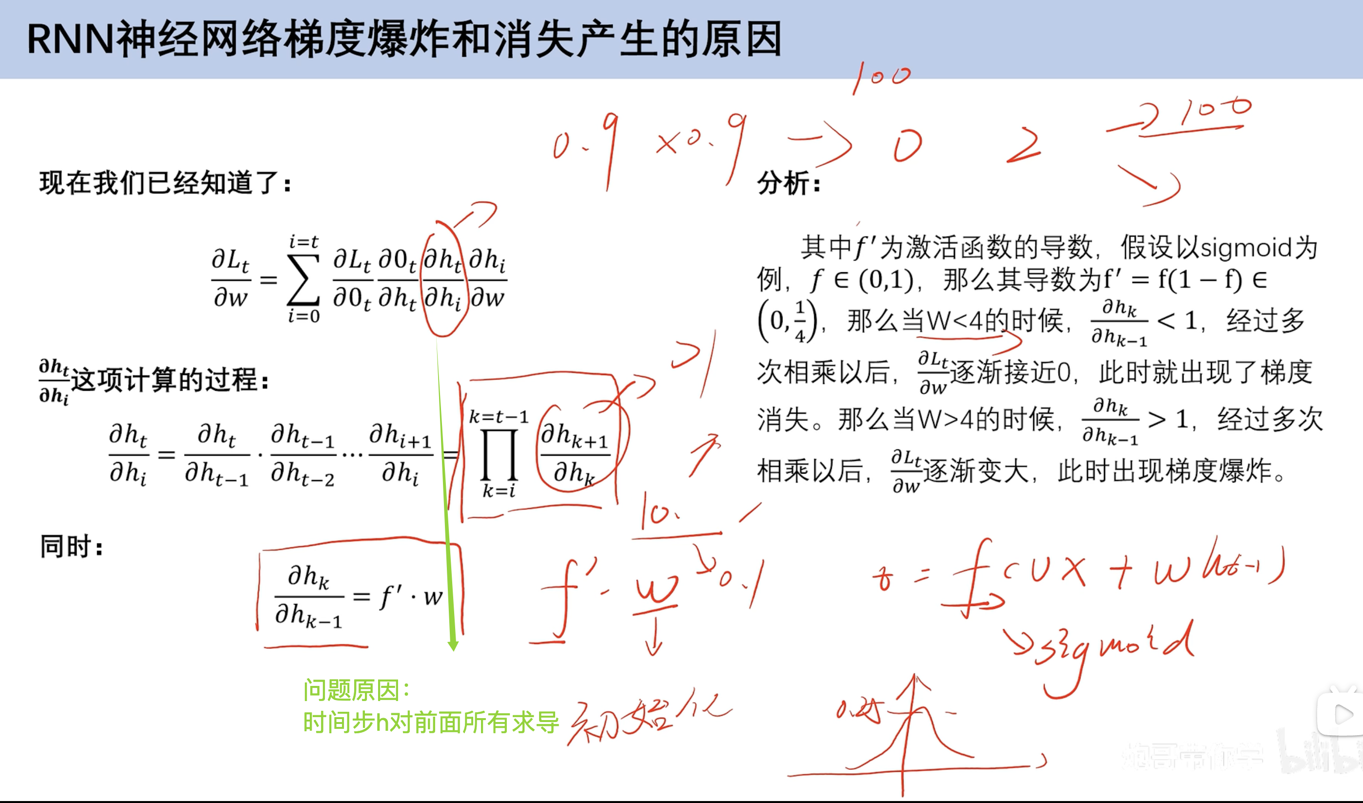
梯度消失和梯度爆炸
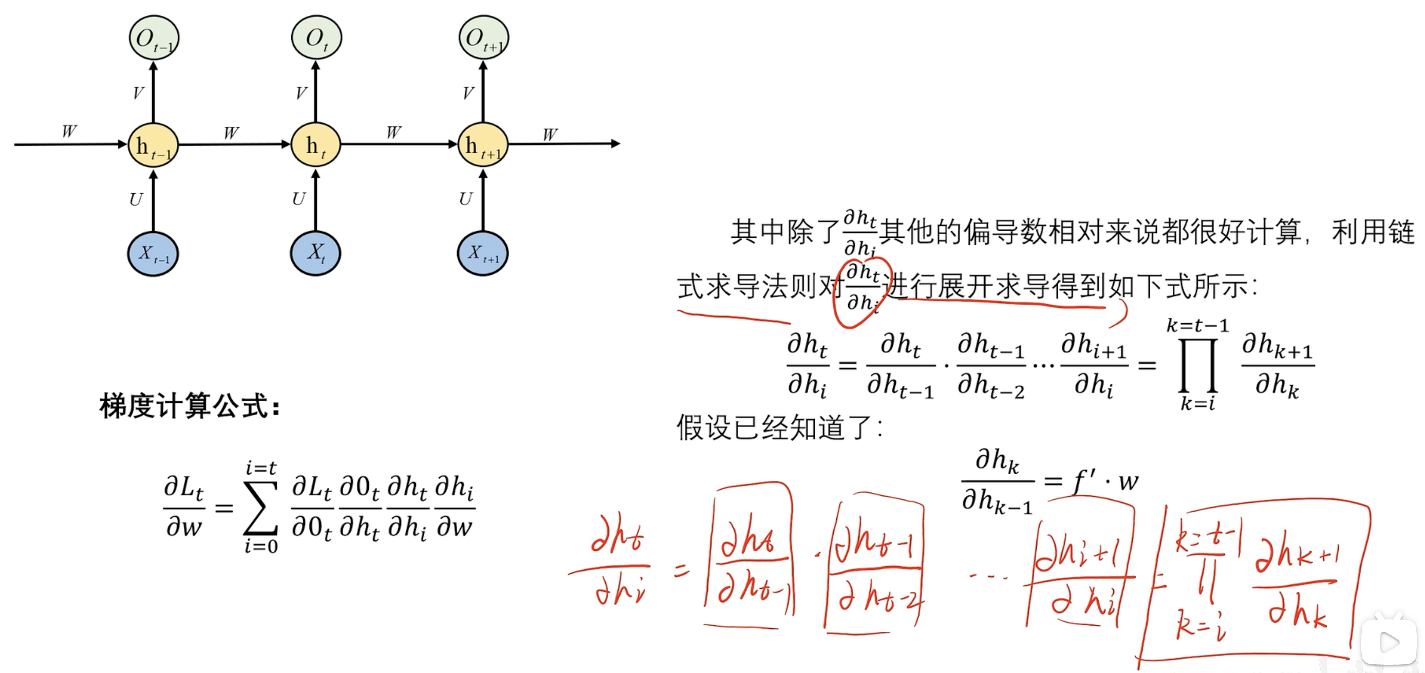
公式
原因
- 假设这里使用sigmoid函数
- 求导后为
f*(1-f)- f=0.5 有最大值1/4
- w共享:
- 所以当w<4 第一个h倒数小于1 累成 梯度消失 (很难学到前面很长时间的权重 LSTM有缓解)
- 所以当w>4 第一个h倒数大于1 累成 梯度爆炸💥
==LSTM==
和RNN对比
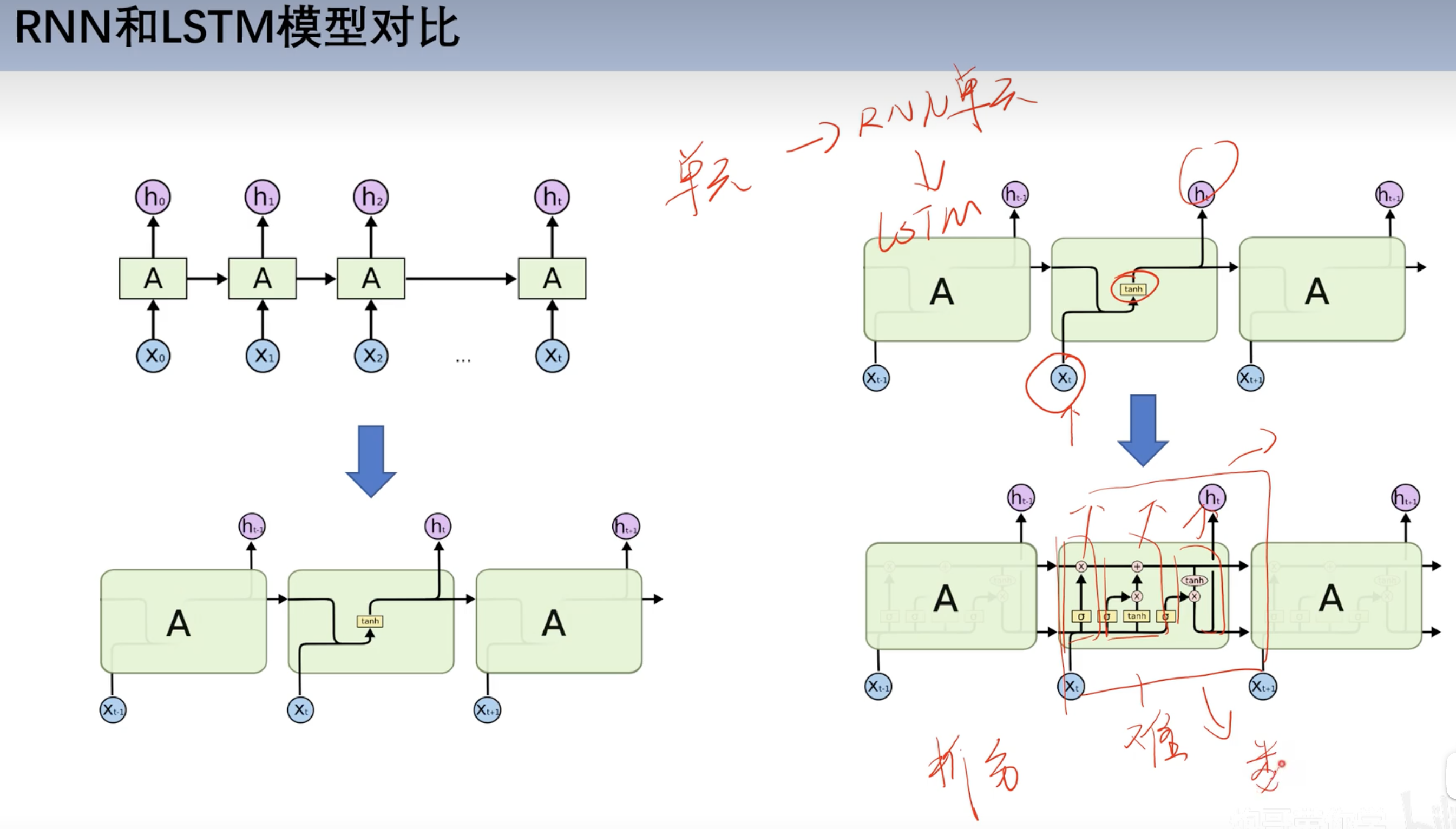
基本结构
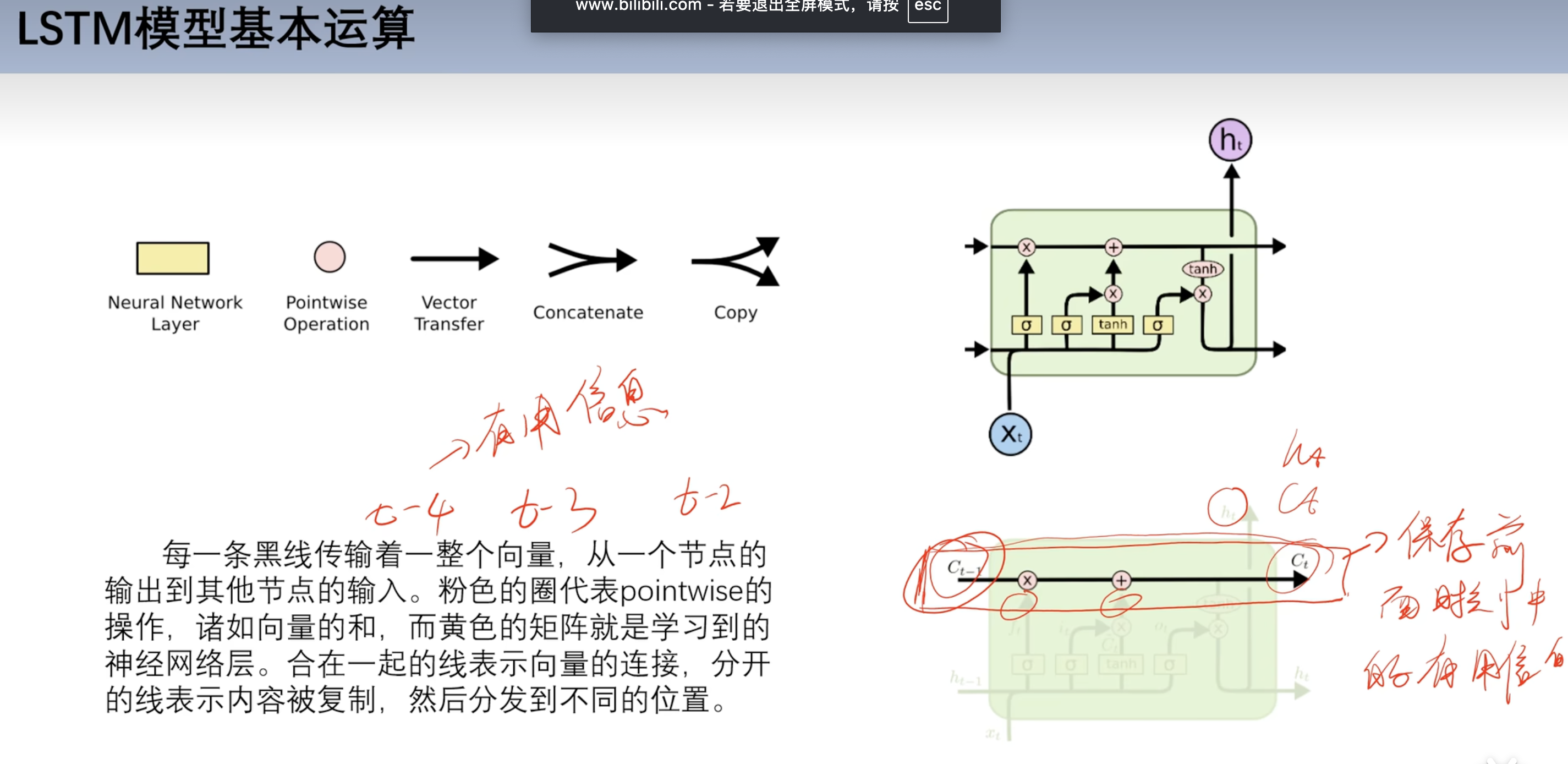
基本运算
- 黄色方框都是激活函数
- 有sigmoid和tanh反双曲正切
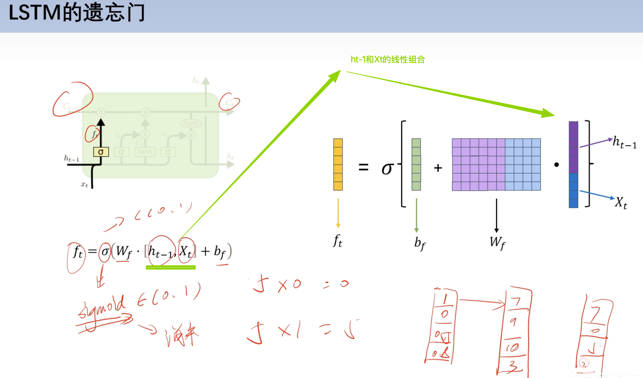
遗忘门
- 作用:保存有用信息,摒弃没用的信息
- 用
sigmoid函数将值域映射在0~1Wf是权重
输入门
结构
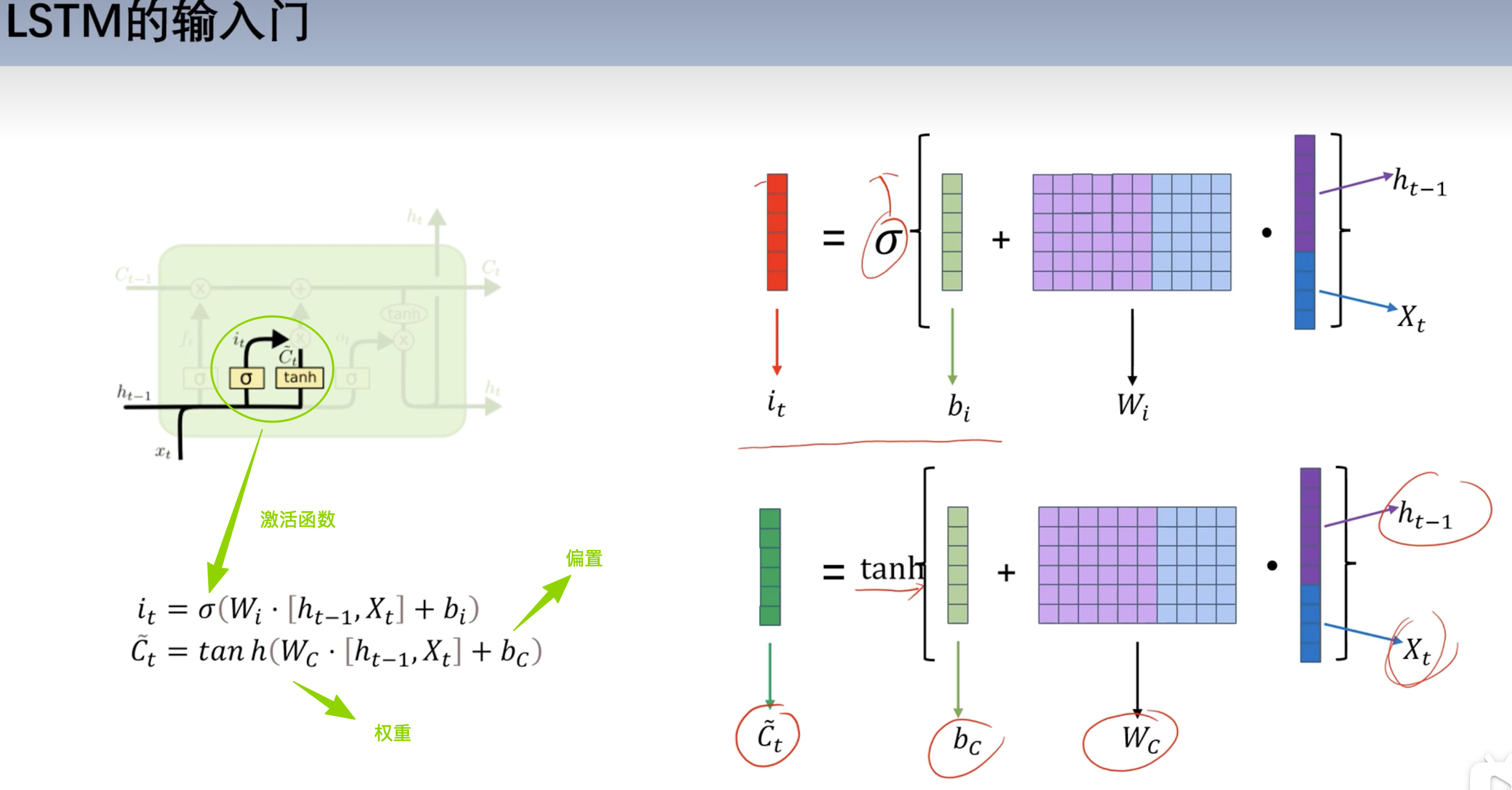
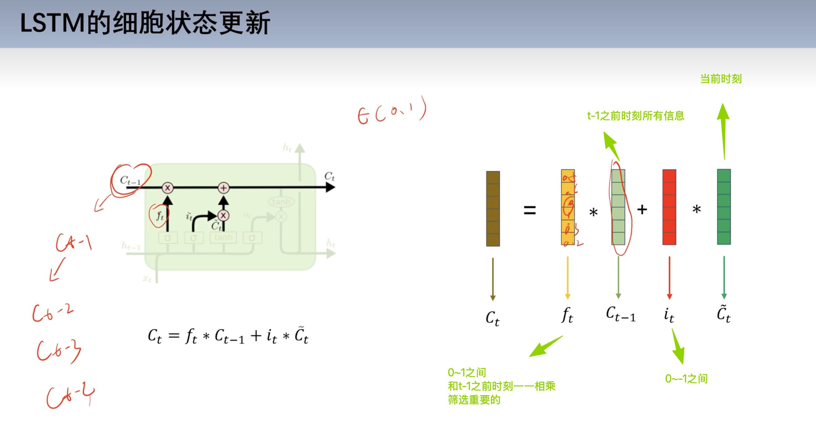
细胞状态更新
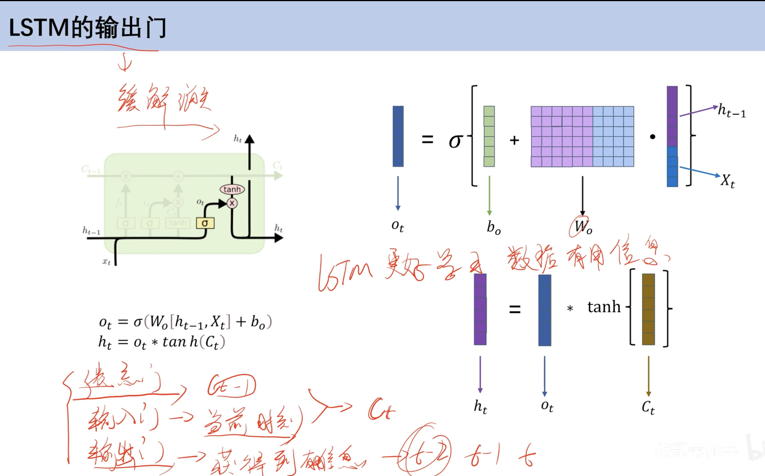
输出门
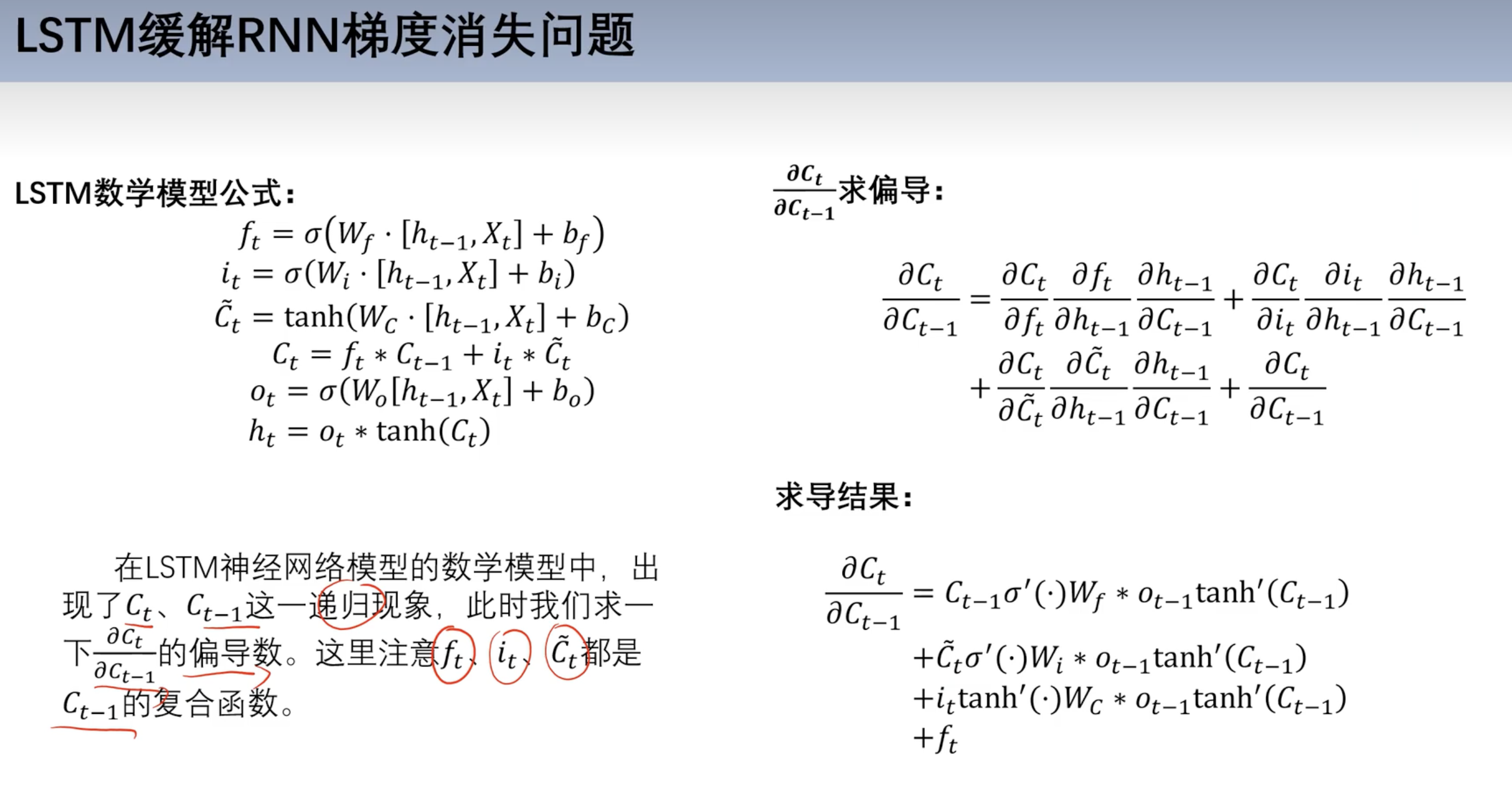
如何缓解梯度消失
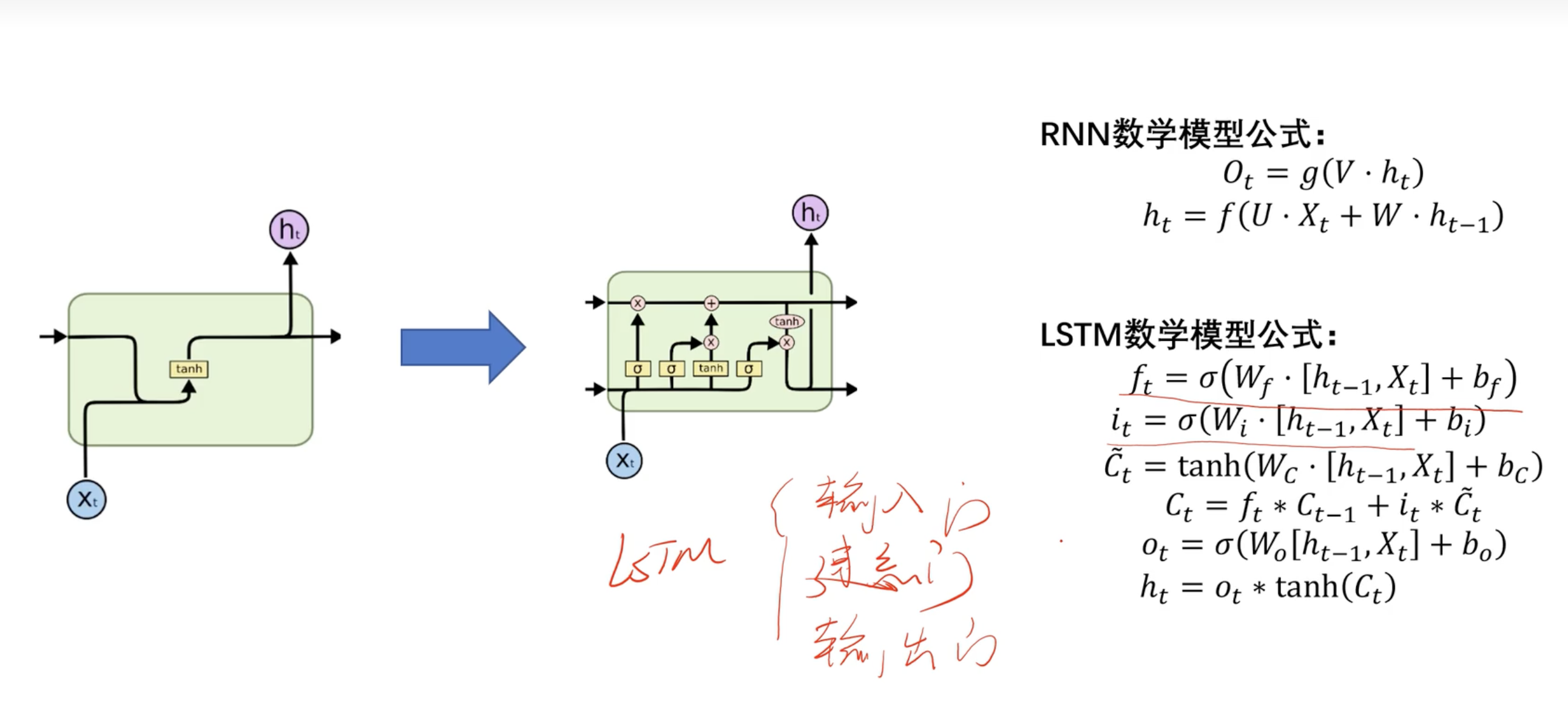
公式对比
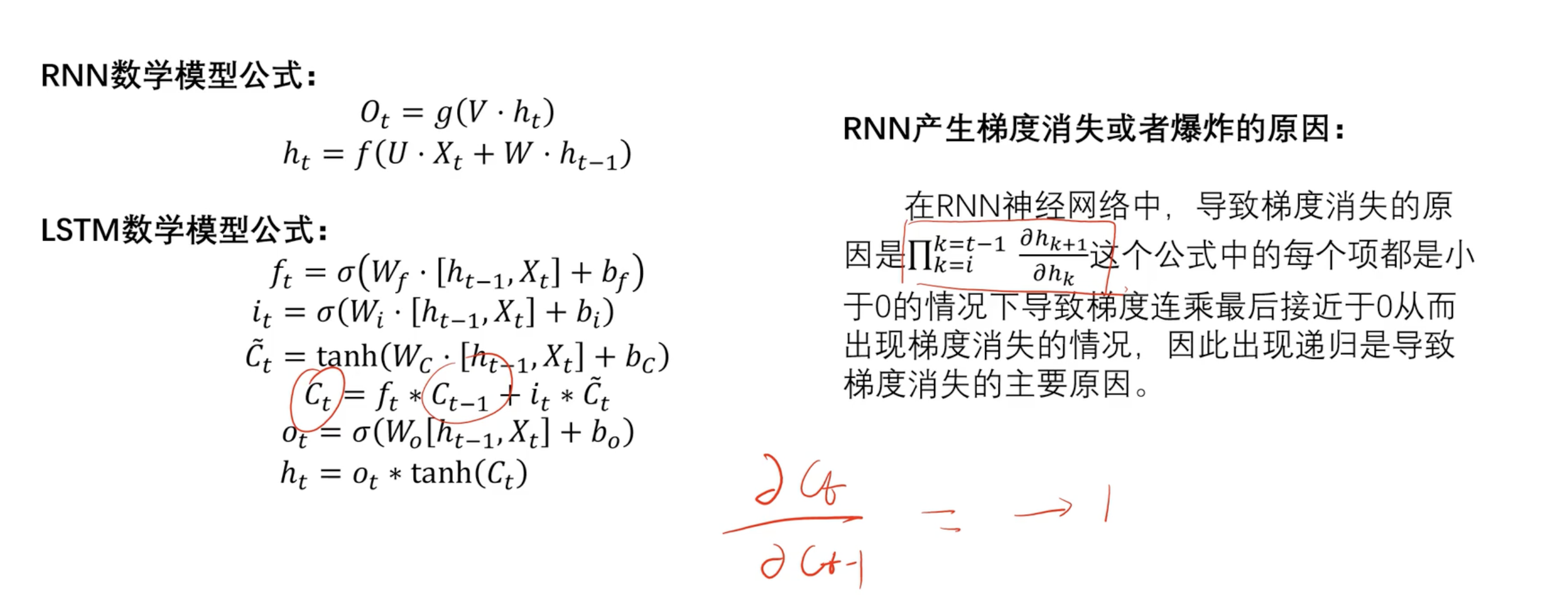
求导
- 对Ct-1 求导
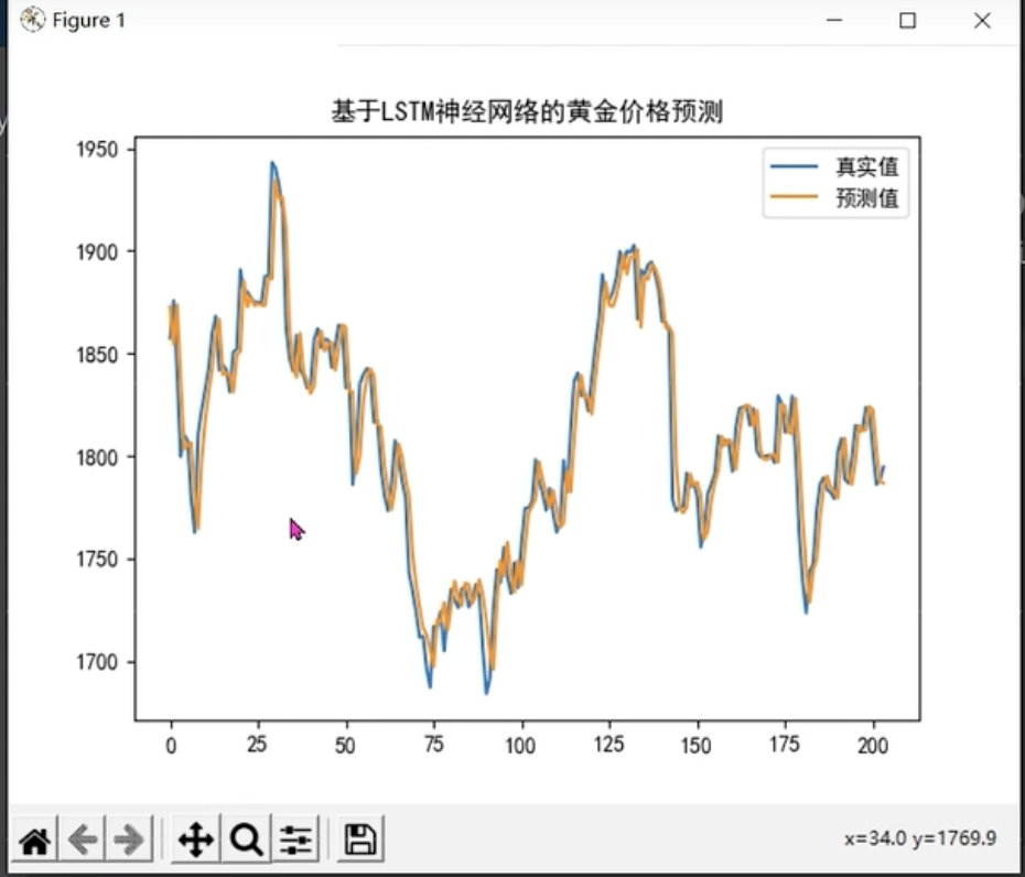
实战(黄金价格预测)
- 单特征情况
- 时间 价格变为多特征
- 前五天预测第六天 滚动预测
- 时间步为5
model_train
1 | # 导入库 |
model_test
1 | # 导入库 |
本博客所有文章除特别声明外,均采用 CC BY-NC-SA 4.0 许可协议。转载请注明来源 cyt的笔记屋!
 微信
微信 支付宝
支付宝
相关推荐
2025-09-02
机器学习-深度学习入门
教程地址: up**:炮哥带你学 课程名字:[手把手教学]快速带你入门深度学习与实战 简介:入门机器学习和深度学习 网址: https://www.bilibili.com/video/BV1eP411w7Re/?spm_id_from=333.1387.homepage.video_card.click&vd_source=f8d1f5518d3f58b48b5c428323f8d3bf up**:炮哥带你学 课程名字:Pytorch框架与经典卷积神经网络与实战 简介:入门深度学习和pytorch 网址: https://www.bilibili.com/video/BV1e34y1M7wR/?spm_id_from=333.1387.homepage.video_card.click&vd_source=f8d1f5518d3f58b48b5c428323f8d3bf 简介 深度学习以神经网络为基础 神经网络 并非隐藏层越多越好 可能过拟合 全连接神经网络 通过训练w和b(权重和偏置) 注:机器学习内容 神经网络作用...

2025-10-17
小土堆pytorch教程
视频地址:https://www.bilibili.com/video/BV1hE411t7RN Dataset Dataset 获取数据并编号 Dataloader 对数据打包 12345678910111213141516171819202122232425262728293031from torch.utils.data import Dataset, DataLoader import numpy as np from PIL import Image import os from torchvision import transforms from torchvision.utils import make_grid class MyDataset(Dataset): def __init__(self, root_dir, label_dir): self.root_dir = root_dir self.label_dir = label_dir self.path = ...