机器学习-深度学习入门

教程地址：

1. up**：炮哥带你学

课程名字：[手把手教学]快速带你入门深度学习与实战

简介：入门机器学习和深度学习

网址：

https://www.bilibili.com/video/BV1eP411w7Re/?spm_id_from=333.1387.homepage.video_card.click&vd_source=f8d1f5518d3f58b48b5c428323f8d3bf

2. up**：炮哥带你学

课程名字：Pytorch框架与经典卷积神经网络与实战

简介：入门深度学习和pytorch

网址：

https://www.bilibili.com/video/BV1e34y1M7wR/?spm_id_from=333.1387.homepage.video_card.click&vd_source=f8d1f5518d3f58b48b5c428323f8d3bf

简介

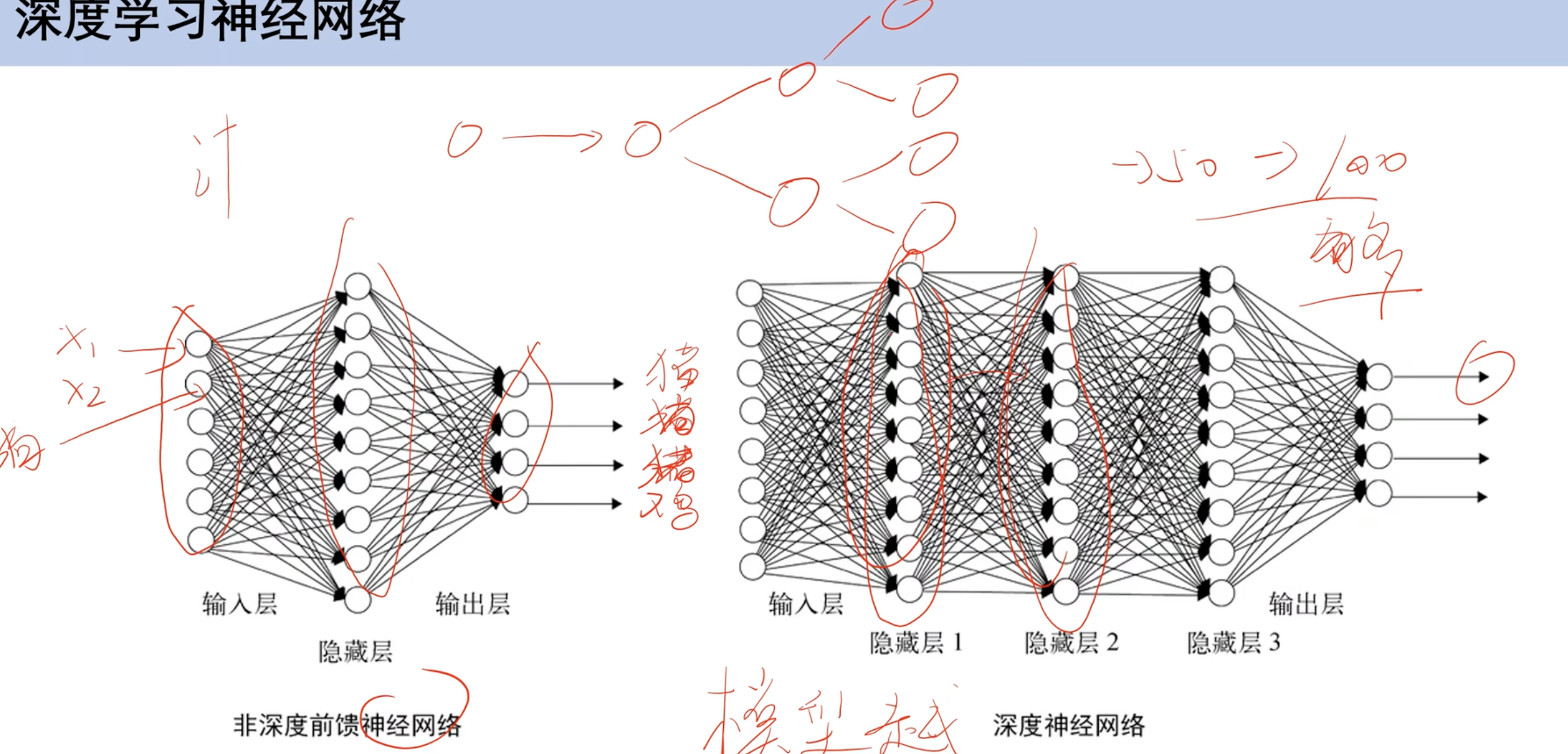
深度学习以神经网络为基础

神经网络

• 并非隐藏层越多越好 可能过拟合

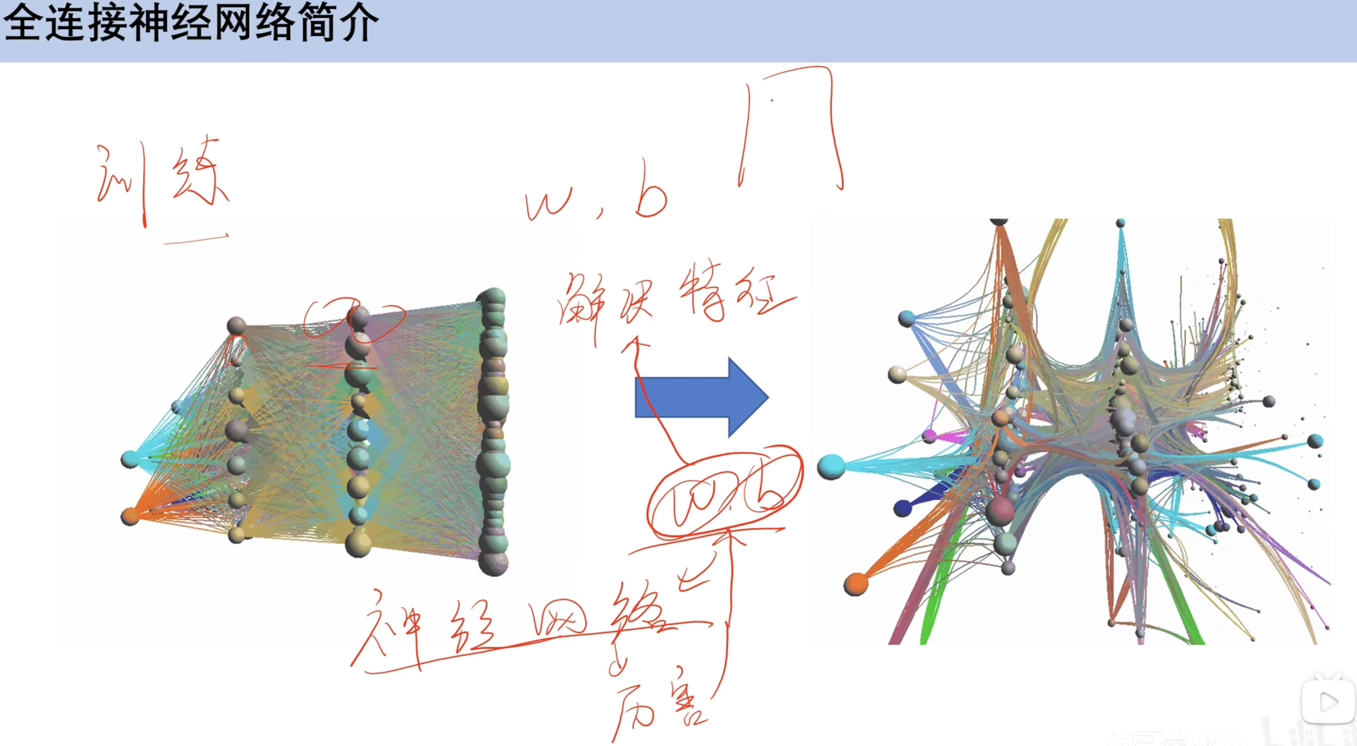
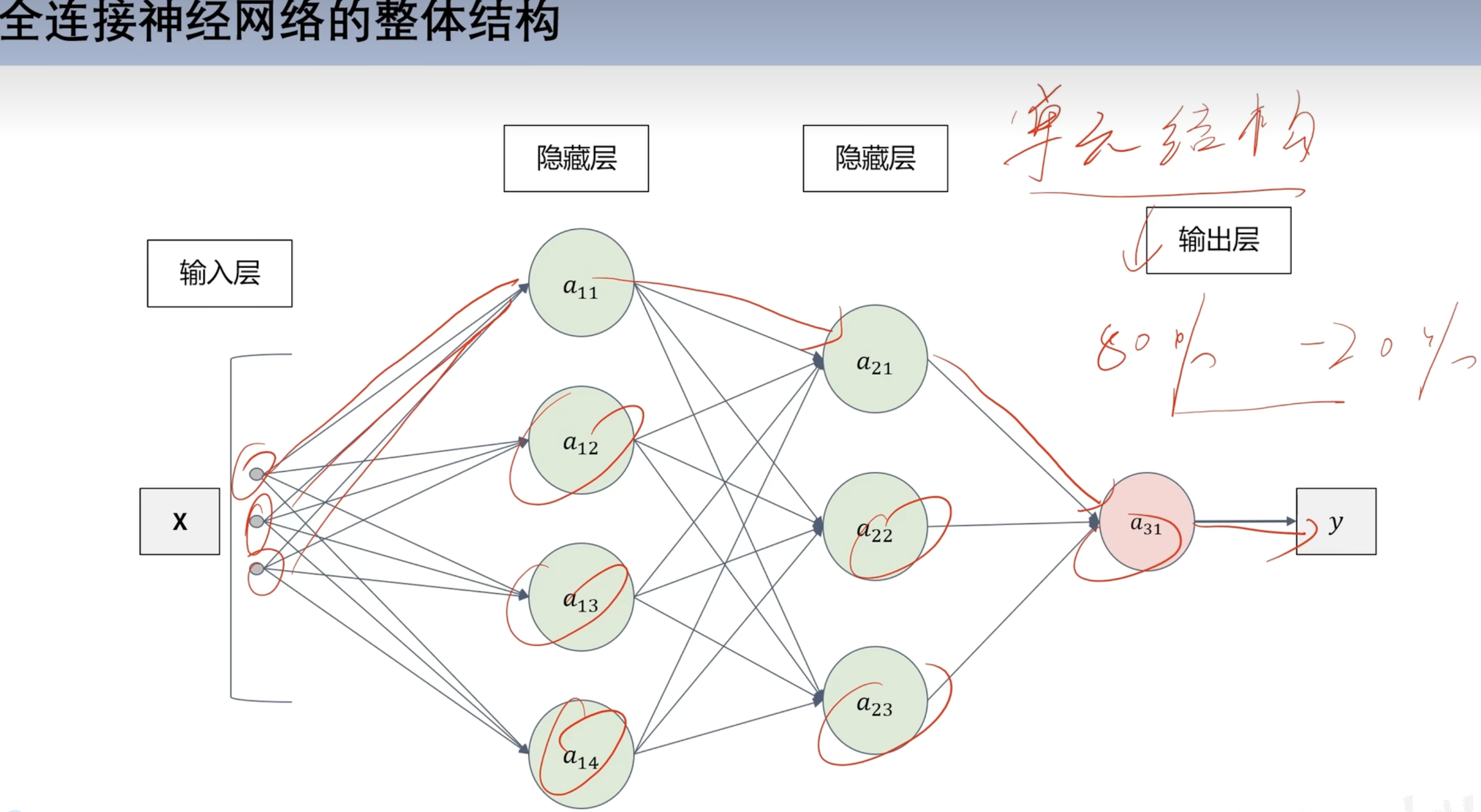
全连接神经网络

通过训练w和b（权重和偏置）

• 注：机器学习内容

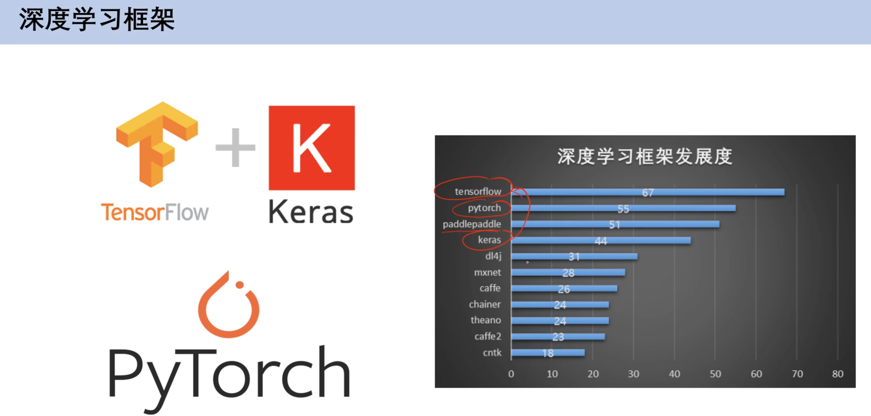
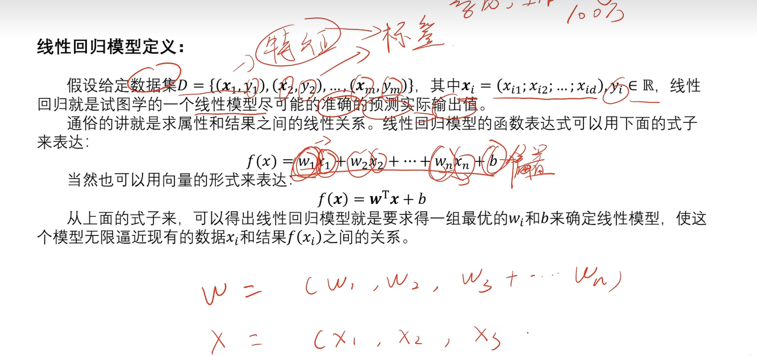
神经网络作用

==深度学习框架介绍==

环境介绍

机器学习知识回顾

2. 线性回归模型与梯度下降

2.2 定义

• x是特征 y是标签

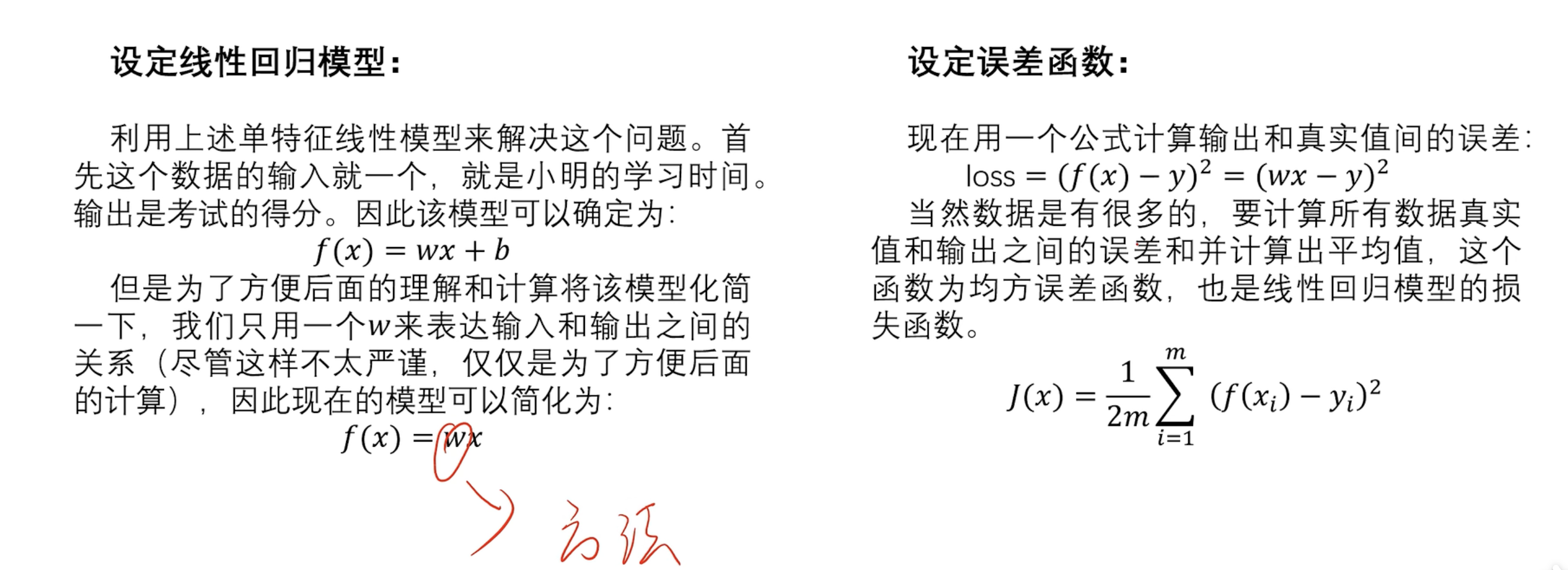
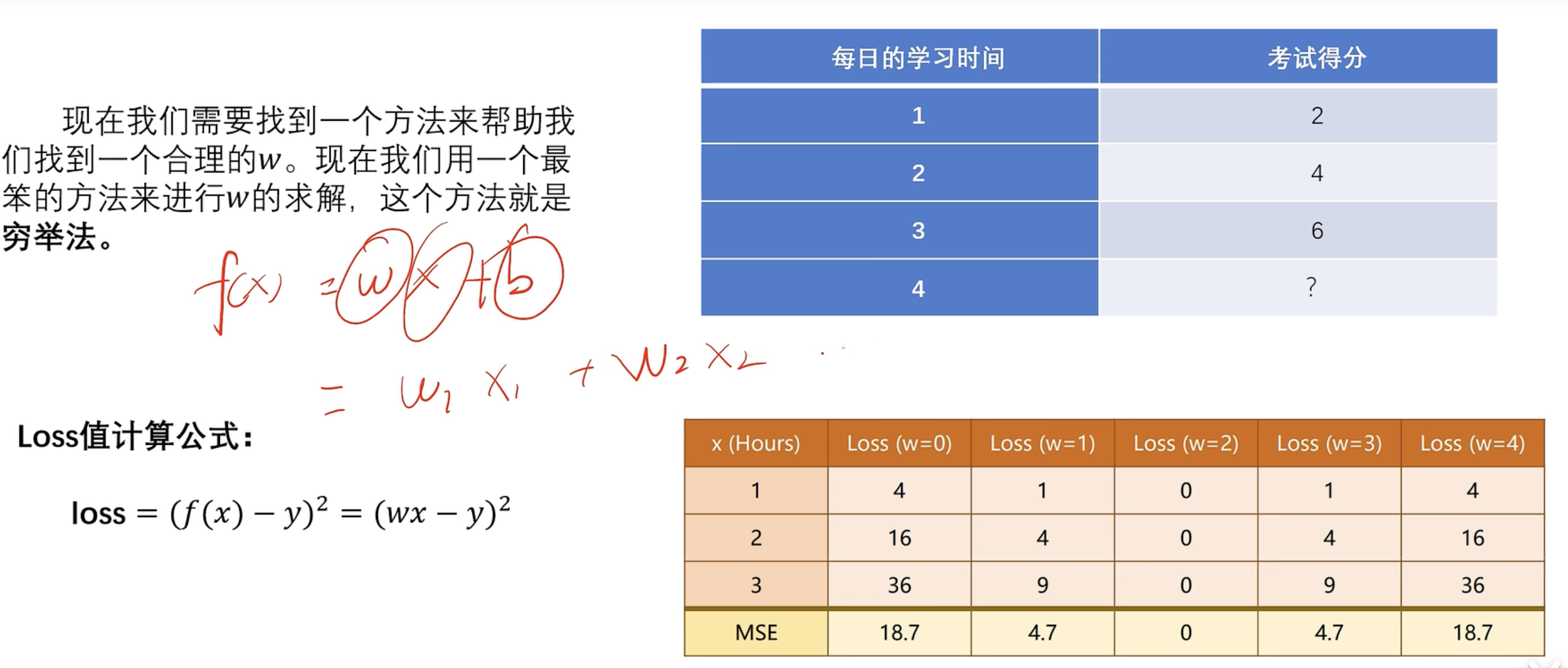
损失函数 （误差函数）

穷举法

• 过于垃圾 看后面最小二乘法

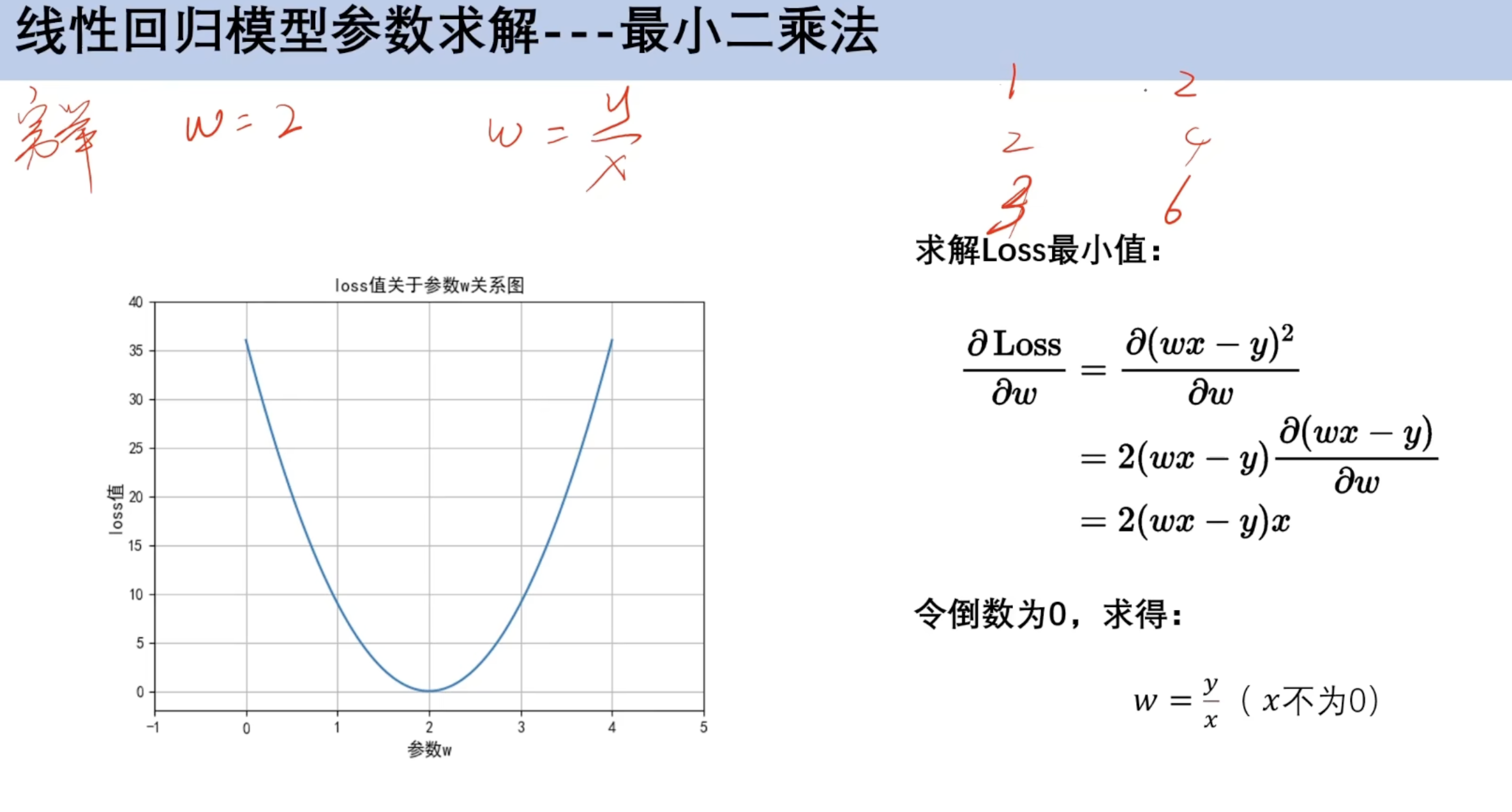
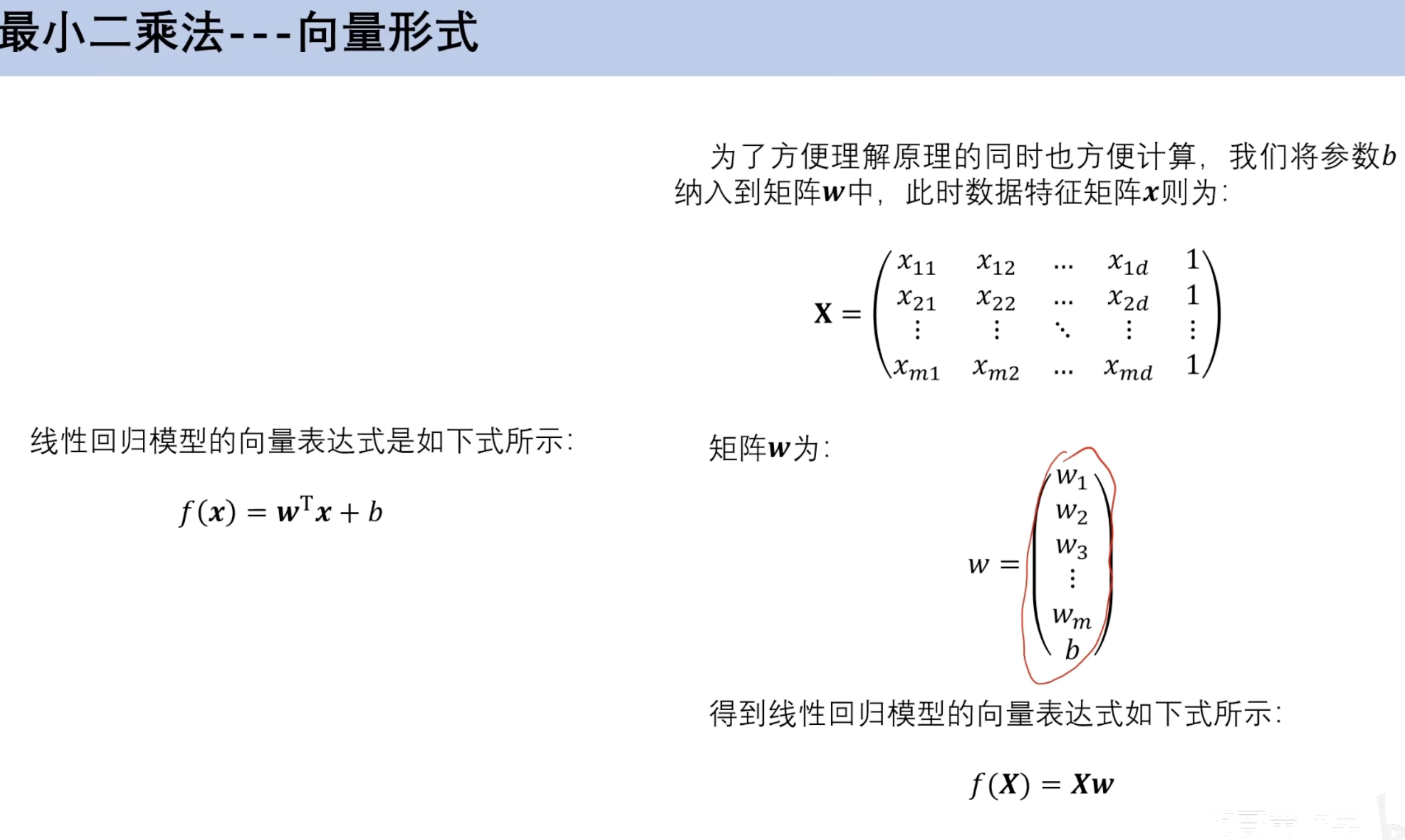
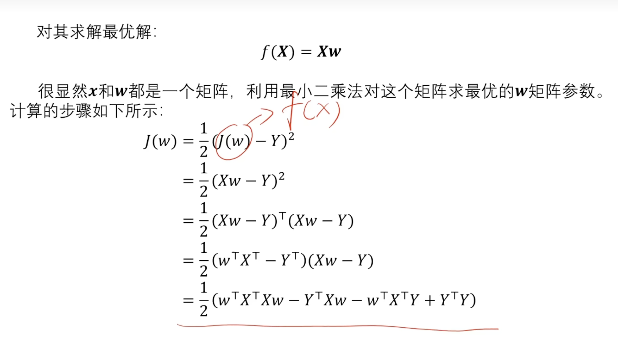
2.3 最小二乘法

对x求偏导

向量版本

• 损失函数
• 更正 此处J（W）为f（x）

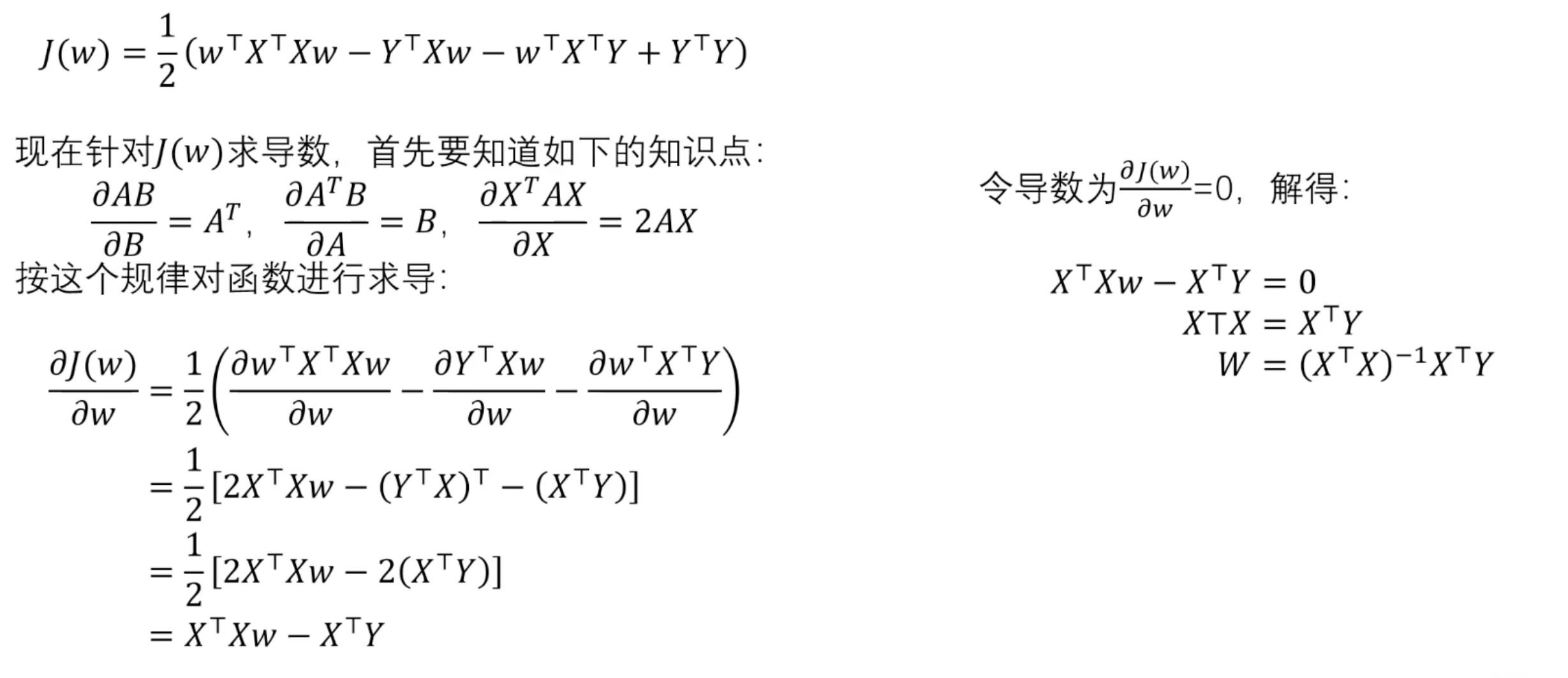
• 对损失函数求导
• 并非所有矩阵有可逆矩阵，因此引入损失函数

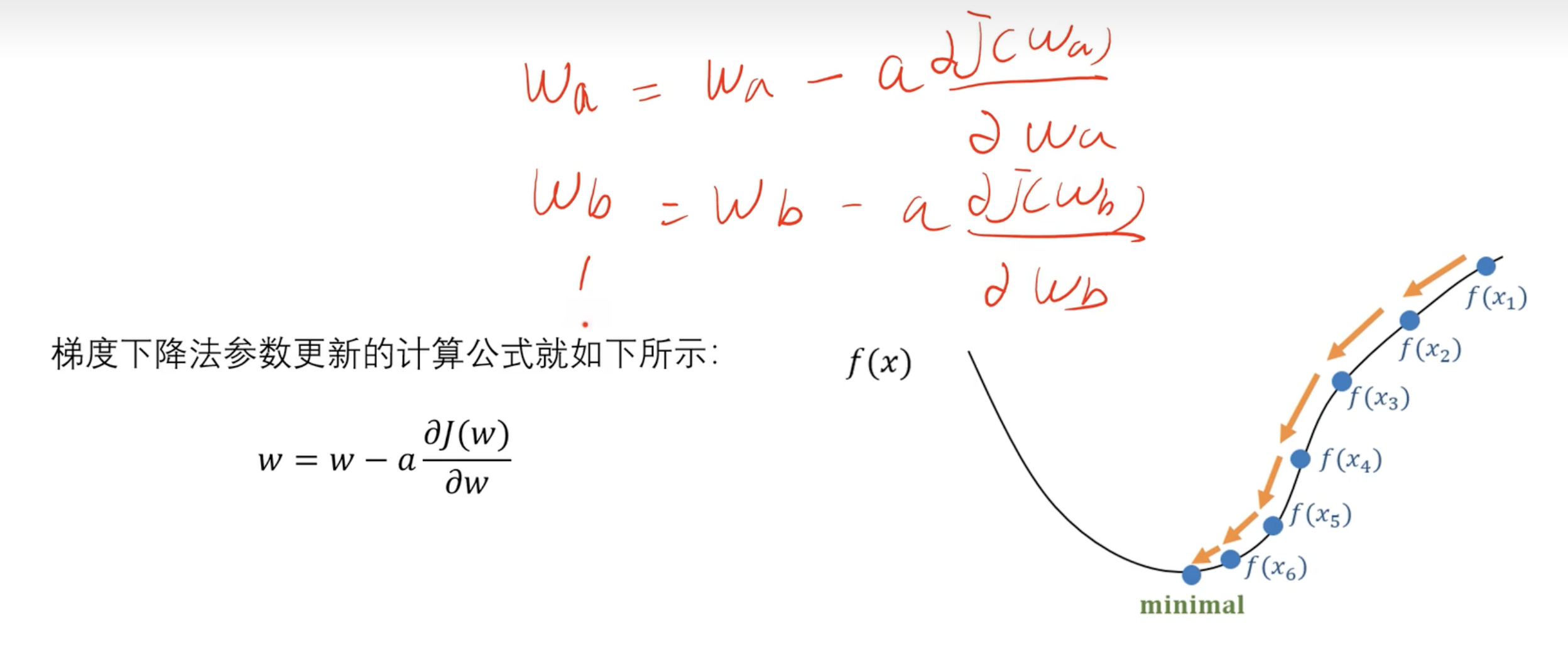
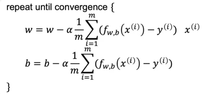
==2.3 梯度下降==

理解

公式

$$
w=w-a \frac{\partial J(w)}{\partial w}
$$

• 对多个w重复计算

• 简化版本

• $$
  \begin{array}{l}
  \text { repeat until convergence { }\
  \begin{aligned}
  w & =w-\alpha \frac{1}{m} \sum_{i=1}^{m}\left(f_{w, b}\left(x^{(i)}\right)-y^{(i)}\right) x^{(i)} \
  b & =b-\alpha \frac{1}{m} \sum_{i=1}^{m}\left(f_{w, b}\left(x^{(i)}\right)-y^{(i)}\right)
  \end{aligned}
  \end{array}
  $$

案例

实战案例

步骤：

1. 数据
2. 模型
3. 损失函数
4. 梯度求导
5. 利用梯度更新参数
6. 设置训练轮次

# 定义数据集

# 定义数据特征
x_data = [1, 2, 3]

# 定义数据标签
y_data = [2, 4, 6]

# 初始化w参数
w = 4


# 定义线性回归的模型
def forword(x):
    return x * w


# 定义损失函数
def cost(xs, ys):
    costvalue = 0
    for x, y in zip(xs, ys):
        y_pred = forword(x)
        costvalue += (y_pred - y) ** 2
    return costvalue / len(xs)


# 定义计算梯度的函数
def gradient(xs, ys):
    grad = 0
    for x, y in zip(xs, ys):
        grad += 2 * x * (forword(x) - y)
    return grad / len(xs)


# 学习率
aa = 0.01

for epoch in range(100):
    cost_val = cost(x_data, y_data)
    gra_val = gradient(x_data, y_data)
    w = w - aa * gra_val
    print('训练轮次：', epoch, 'w=', w, 'loss:', cost_val)

print('100轮后w已经训练好了', 'w=', w)
print("学习4小时最终得分为：", forword(4))

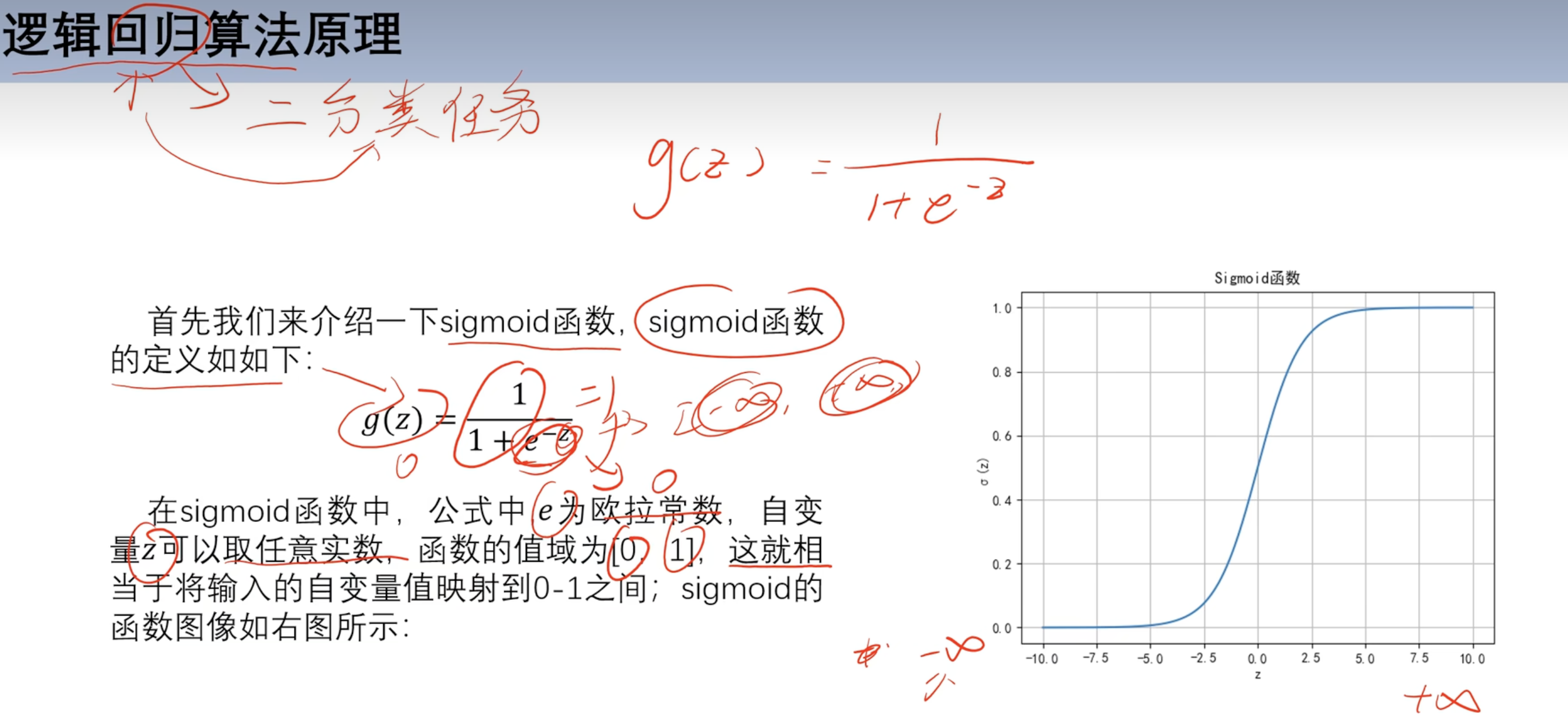
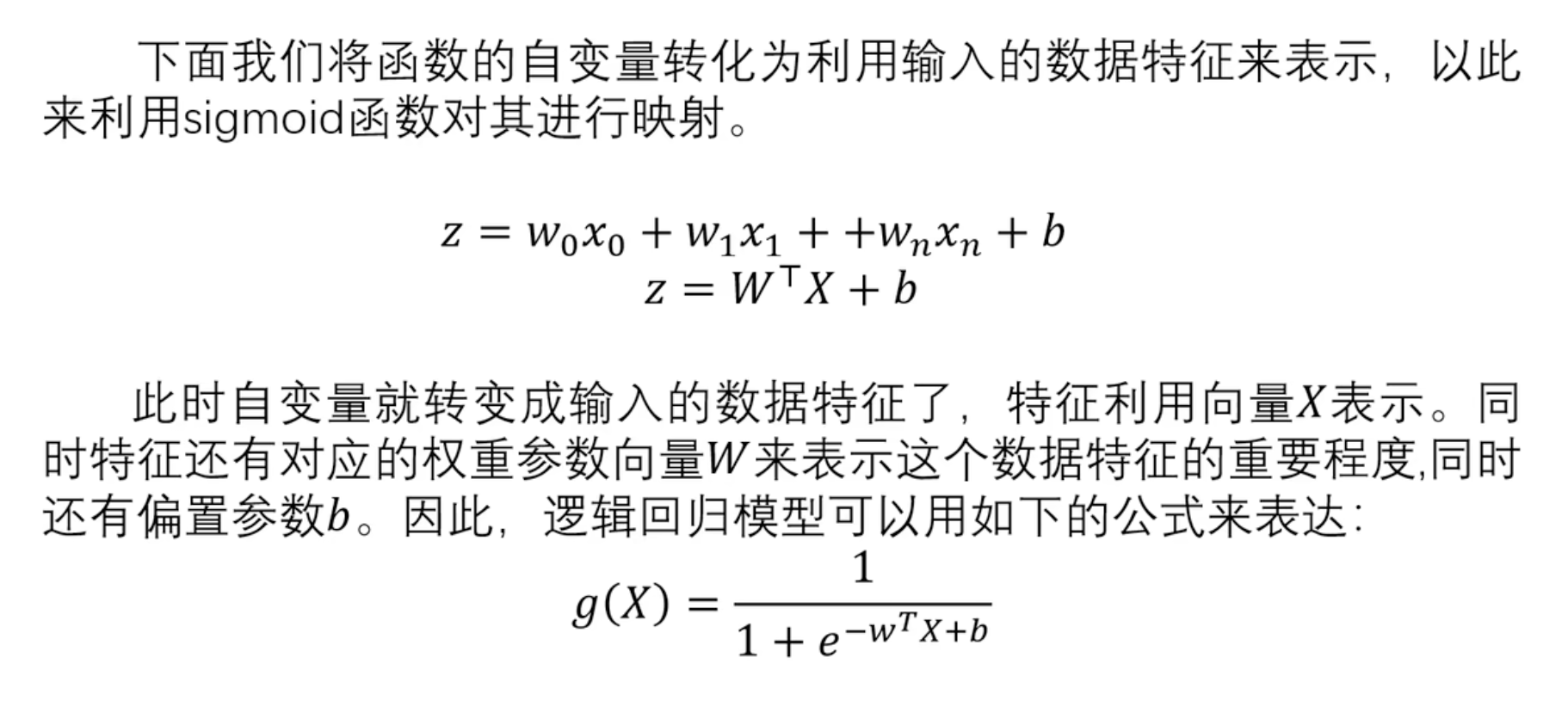
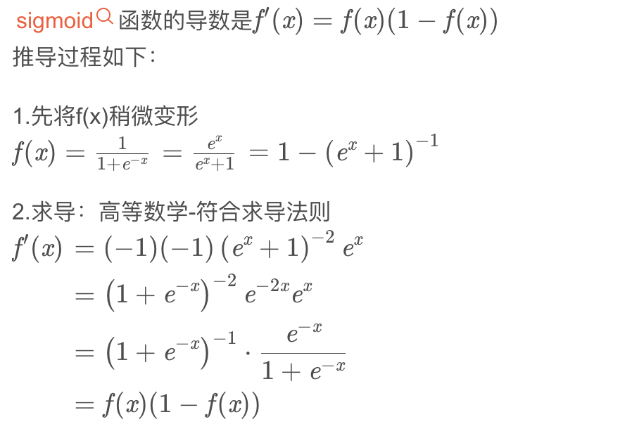
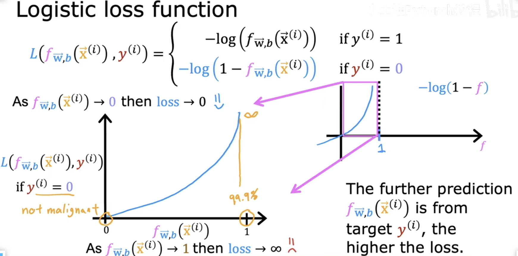
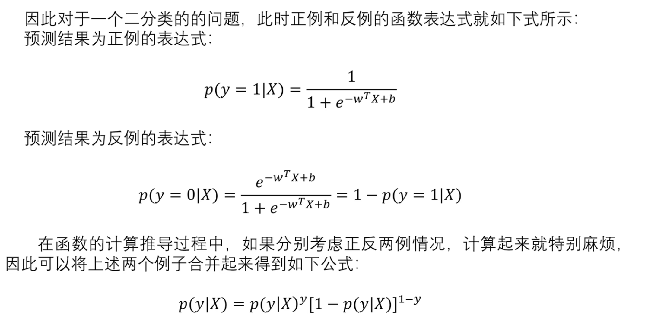
==3.逻辑回归==

3.1 回归和分类的区别

3.2 sigmoid函数

求导

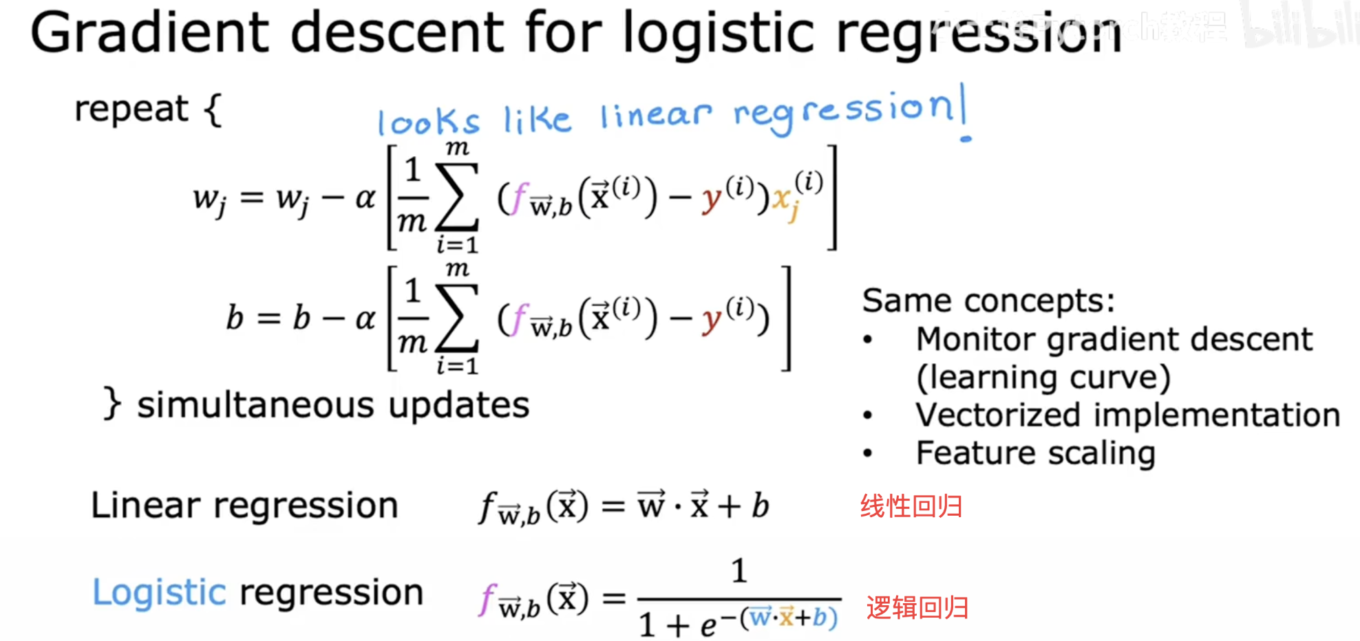
==3.3 损失函数==

表达式

==3.4 梯度下降==

参数w更新

• 向量求导
• 

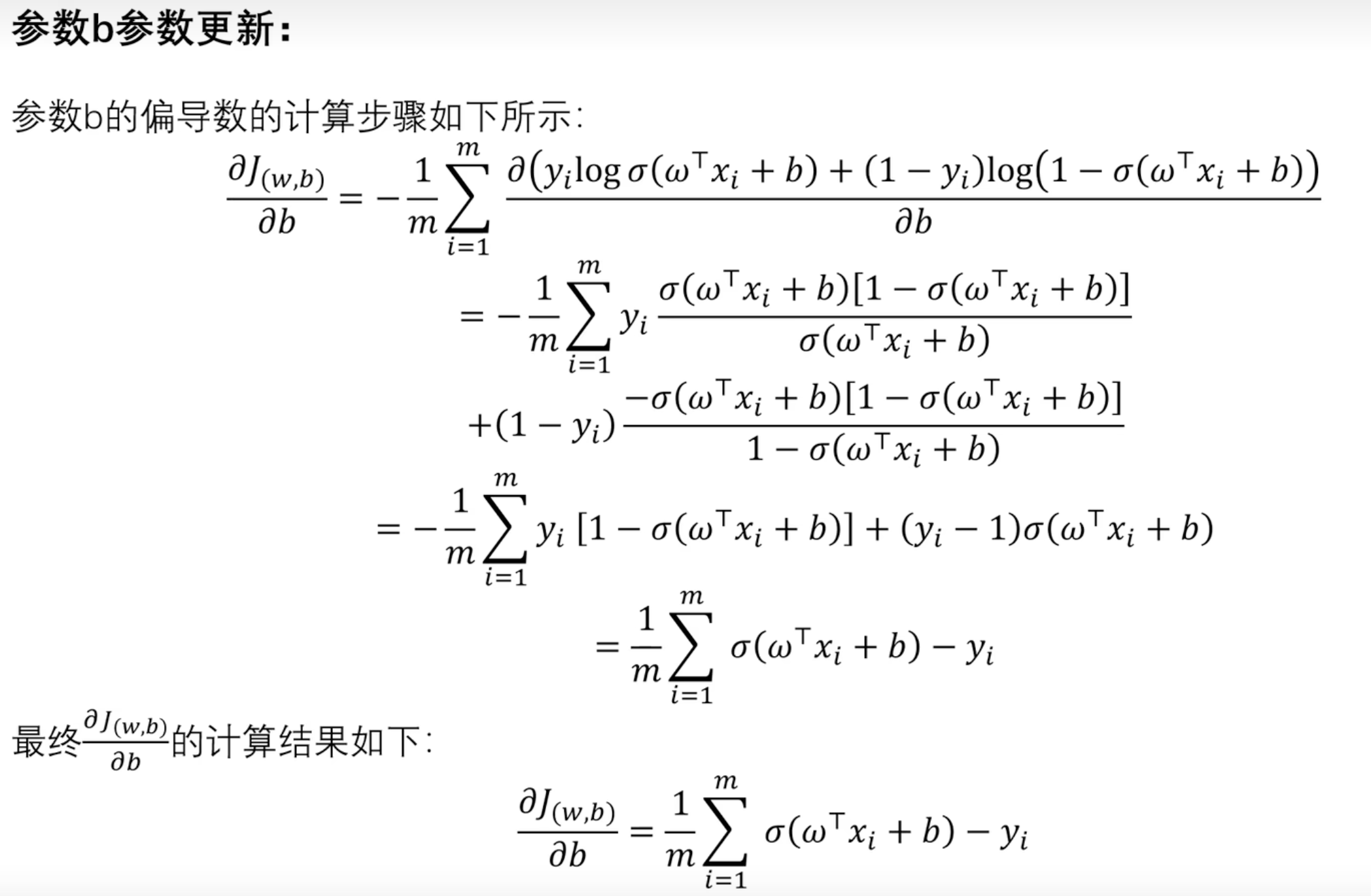
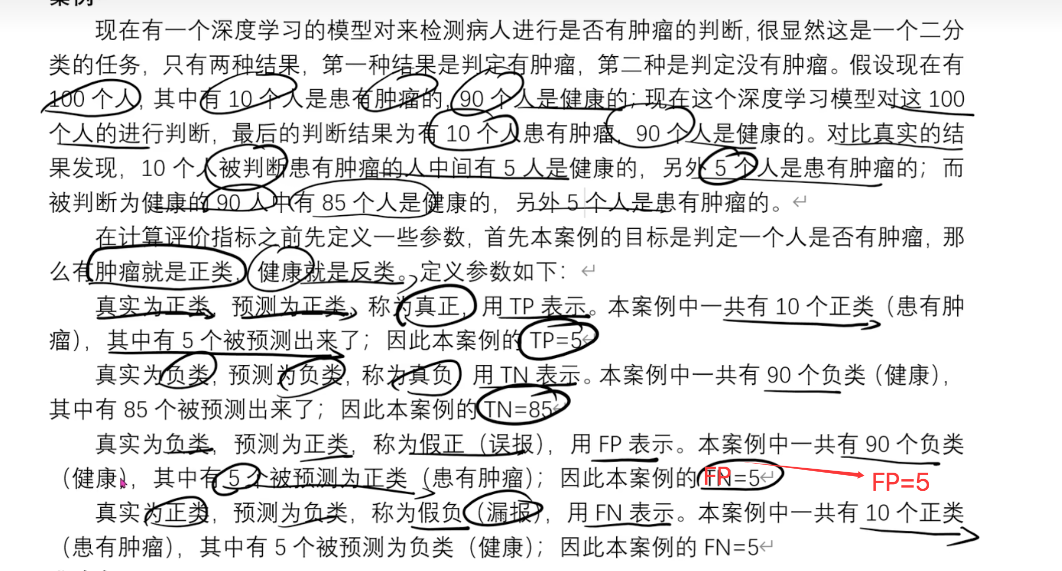
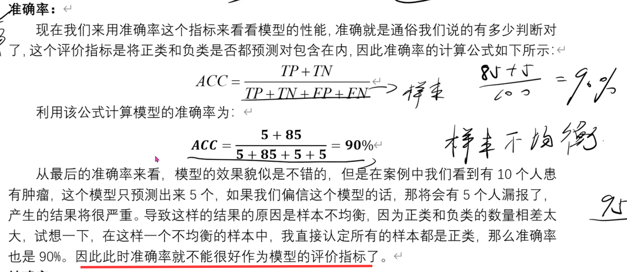
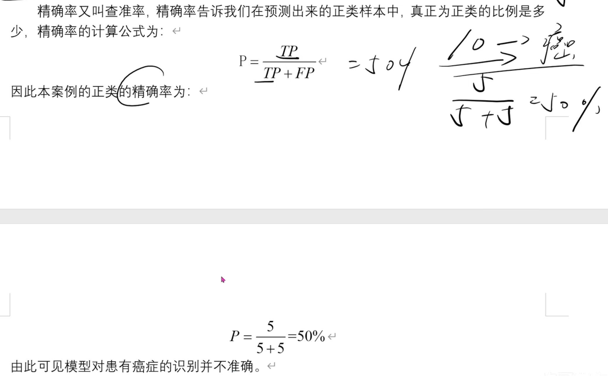
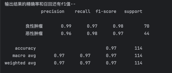
参数b更新

3.5 回归模型评价指标

案例

准确率

精确率

召回率

F1值

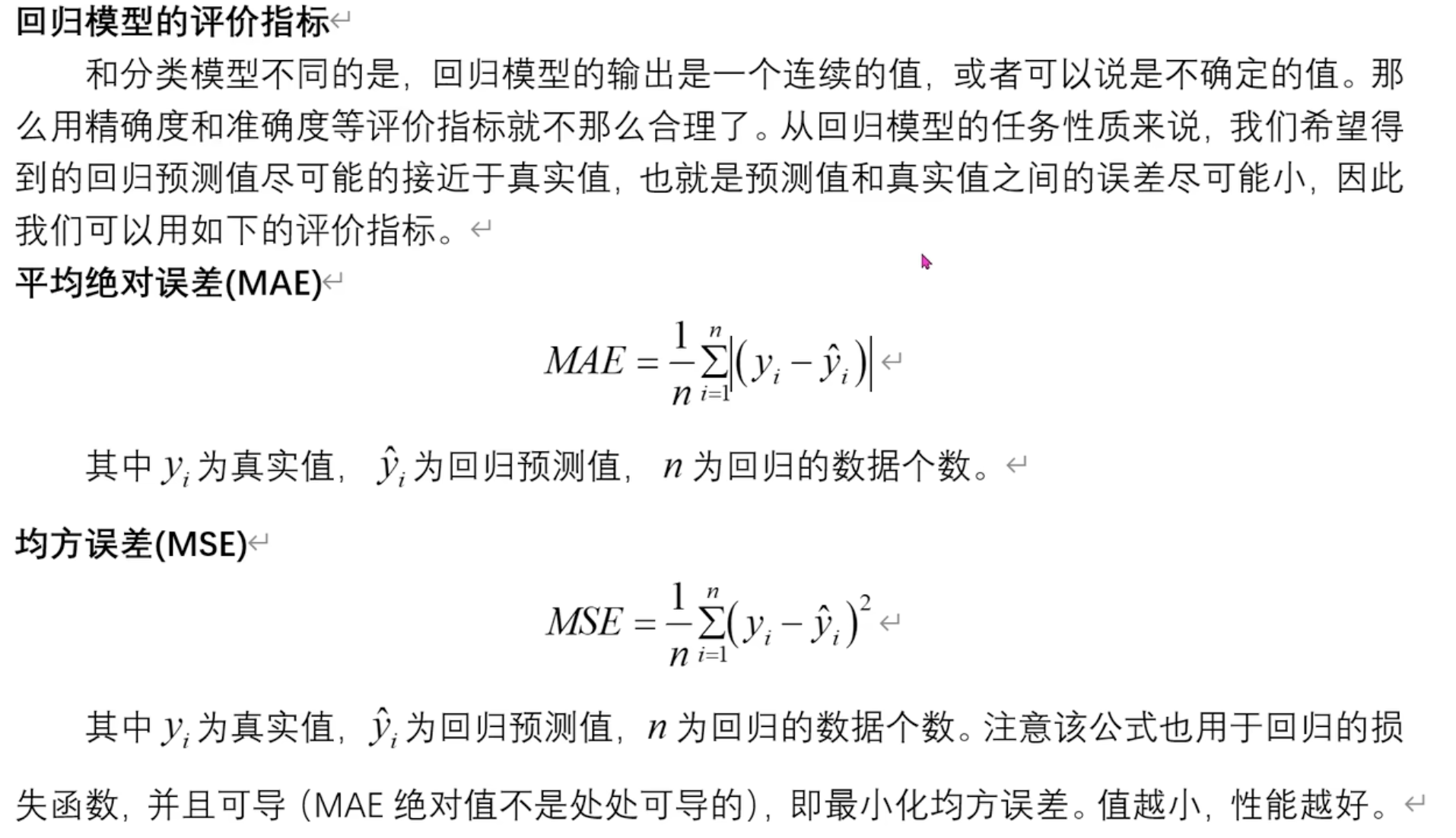
3.6 分类模型评价指标

平均绝对误差（MAE）和==均方误差（MSE）==

MSE 就是前面的LOSS 损失函数

均方根误差（RMSE）

平均绝对百分比误差（MAPE）

3.7 实战案例

代码

1. 归一化公式：(X-min)/(max-min)，消除量纲和数值大小对结果的影响

import numpy as np
import matplotlib.pyplot as plt
import pandas as pd
from sklearn.model_selection import train_test_split
from sklearn.preprocessing import MinMaxScaler
from sklearn.linear_model import LogisticRegression
from sklearn.metrics import classification_report

# 1. 读取数据
dataset = pd.read_csv("breast_cancer_data.csv")
# print(dataset)

# 2.提取特征x
X = dataset.iloc[:, :-1]  # 除了最后一列
# print(x)

# 3.提取数据中的标签
Y = dataset['target']
# print(y)

# 4.划分数据集和测试集 八份训练集 二份测试集 随机抽取
x_train, x_test, y_train, y_test = train_test_split(X, Y, test_size=0.2)

# 5. 数据归一化 使数据在0~1之间 消除量纲影响
sc = MinMaxScaler(feature_range=(0, 1))
x_train = sc.fit_transform(x_train)
x_test = sc.transform(x_test)
# print(x_train)
# print(x_test)

# 6.逻辑回归模型搭建
lr = LogisticRegression()
lr.fit(x_train, y_train)

# 7.打印参数w和b
print("w", lr.coef_)
print("b", lr.intercept_)

# 8. 用训练好的模型推理测试
pre_result = lr.predict(x_test)
print("预测结果：", pre_result)

# 9.打印预测结果的概率
pre_result_proba = lr.predict_proba(x_test)
print("概率：", pre_result_proba)

# 10.获取恶性肿瘤的概率
pre_list = pre_result_proba[:, 1]
print(pre_list)

# 11. 设置保存结果的列表
result = []
result_name = []

# 设置阈值
thresholds = 0.3

for i in range(len(pre_list)):
    if pre_list[i] > thresholds:
        result.append(1)
        result_name.append("恶性")
    else:
        result.append(0)
        result_name.append("良性")

# 打印阈值调整后结果
print("打印阈值调整后结果:")
print(result)
print(result_name)

# 输出结果的精确率和召回还有f1值
print(y_test)
report = classification_report(y_test, result, labels=[0, 1], target_names=['良性肿瘤', '恶性肿瘤'])
print("输出结果的精确率和召回还有f1值--")
print(report)

结果打印

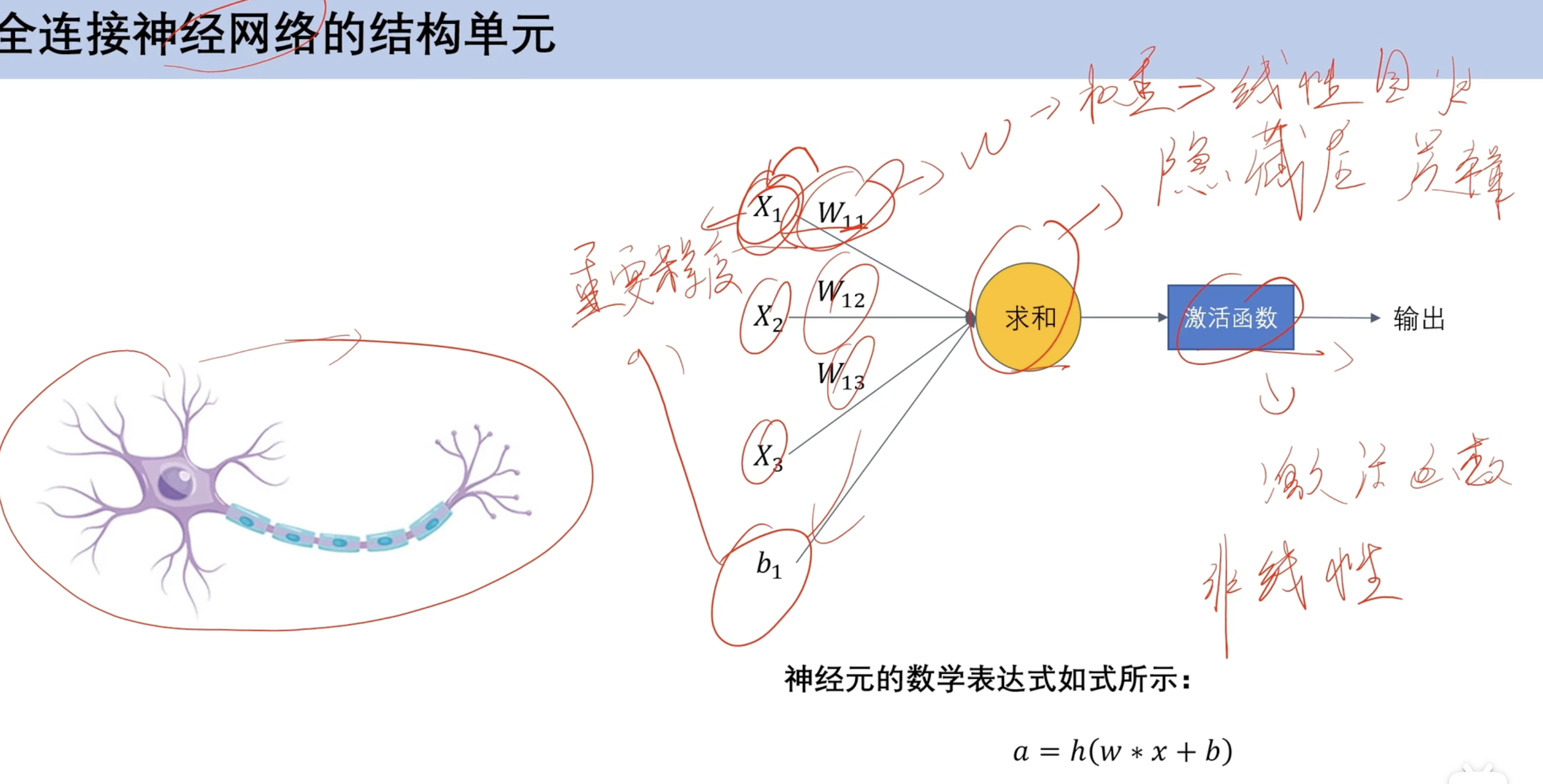
深度学习

全连接神经网络

结构

结构单元

• 类比机器学习回归模型

1. x 输入
2. b 偏置
3. w权重
4. 求和：隐藏层
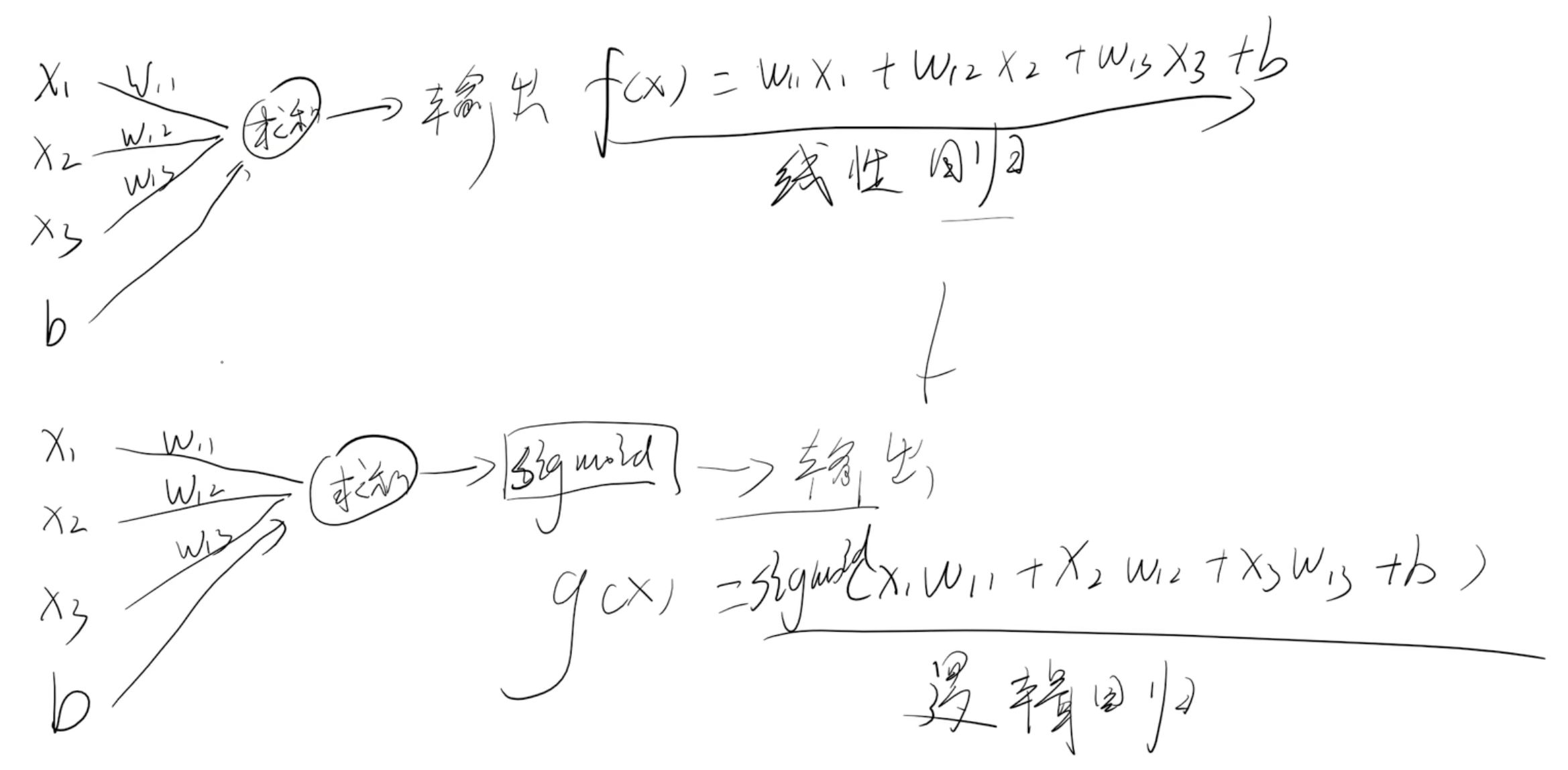
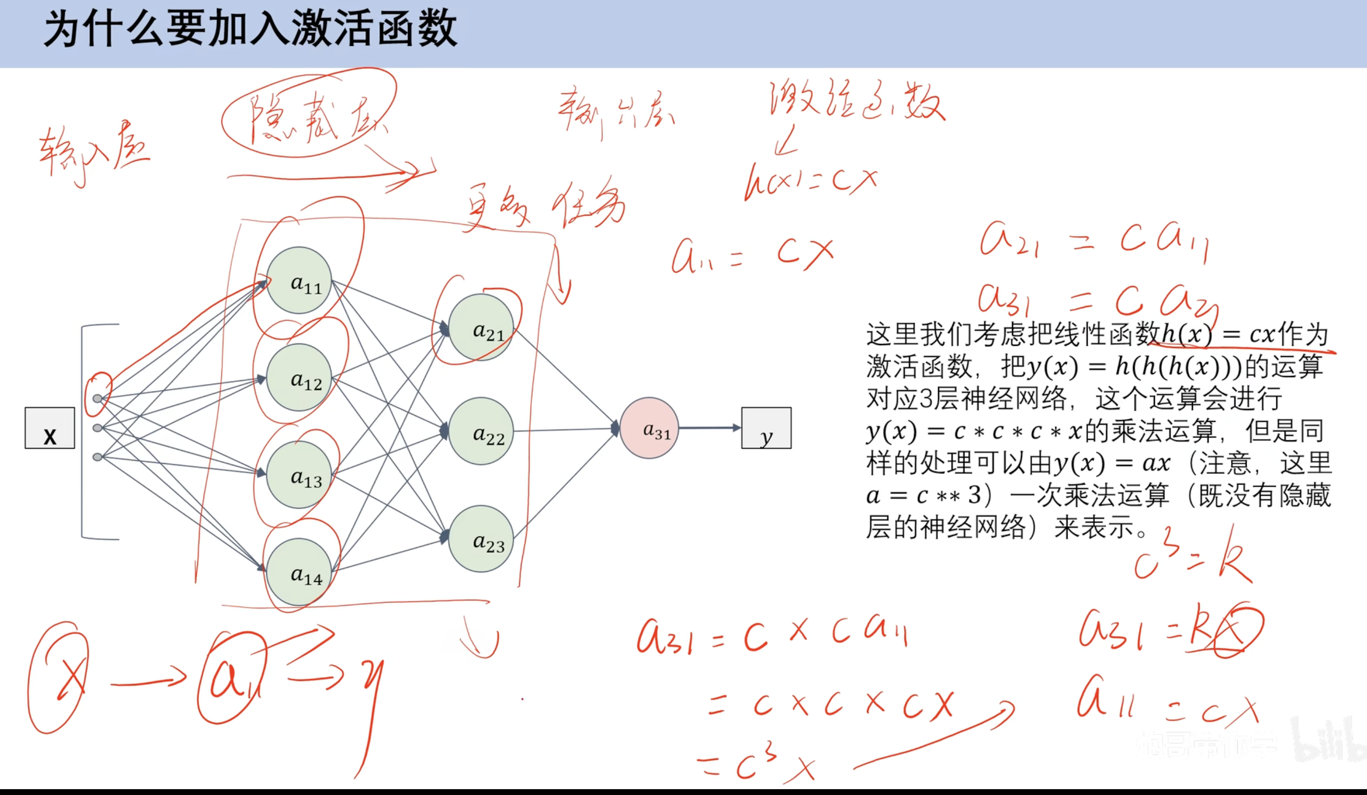
5. 激活函数：非线性 ==（对比逻辑回归激活函数是求和 逻辑回归激活函数是sigmoid）==

对比机器学习激活函数

• 对比逻辑回归激活函数是求和 逻辑回归激活函数是sigmoid）

激活函数作用

• 非线性：这样最后就不会得到c的三次方为常数

激活函数

CSDN: 激活函数图像大全

https://blog.csdn.net/hy592070616/article/details/120617490

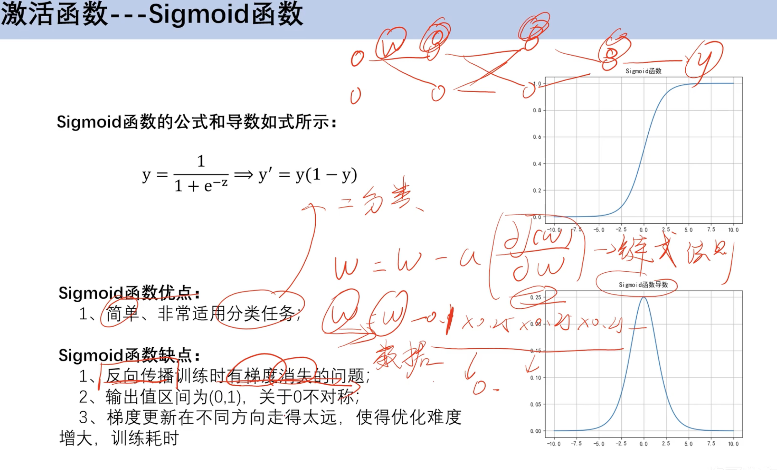
sigmoid函数

• 梯度消失问题，倒数图像左右消失太快 w累计乘法后小数累成 趋近于0

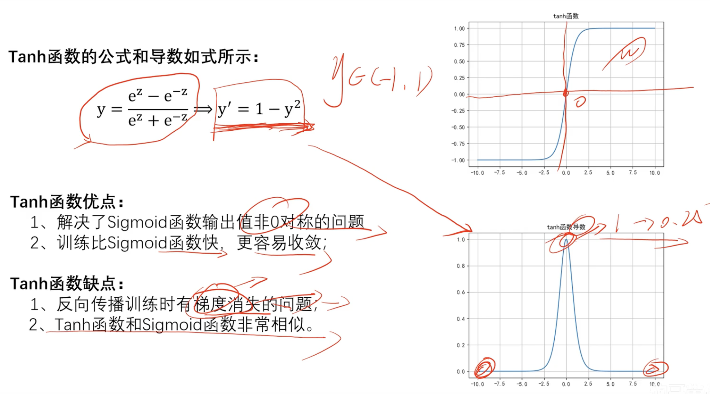
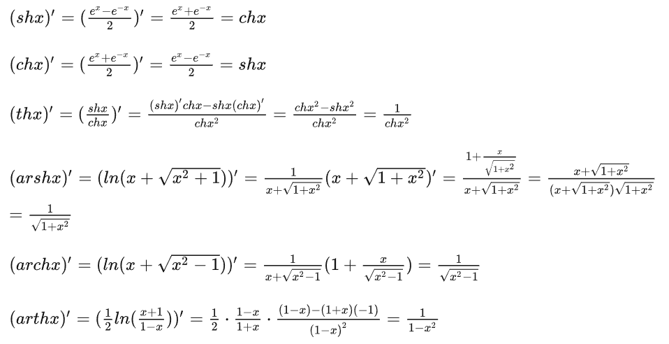
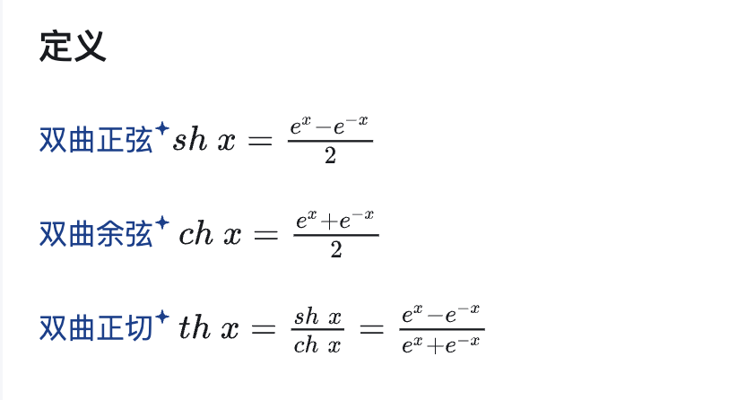
Tanh函数（双曲正切函数）

数学知识

知乎：https://zhuanlan.zhihu.com/p/563840693

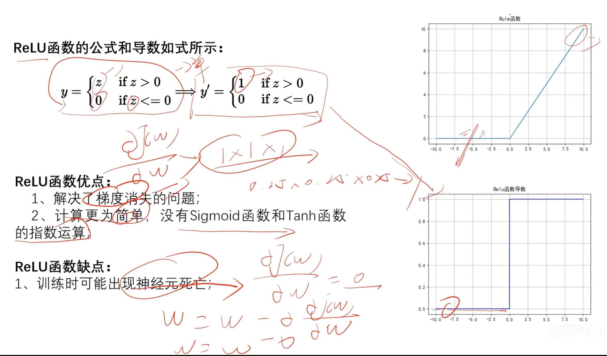
ReLU函数

• 神经元死亡：z<0 倒数为0 w停止更新

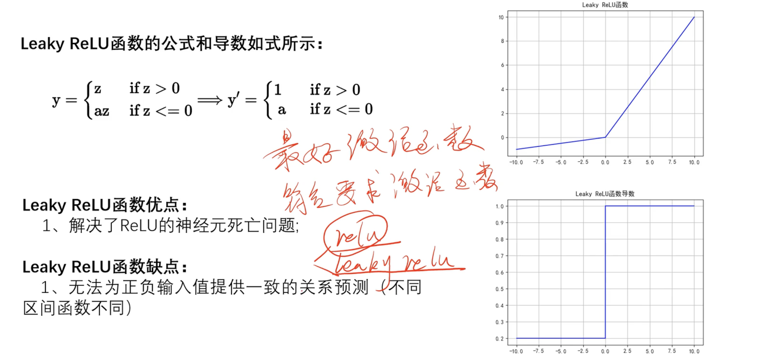
Leaky ReLU

• 没有最好的激活函数 只有符合的激活函数

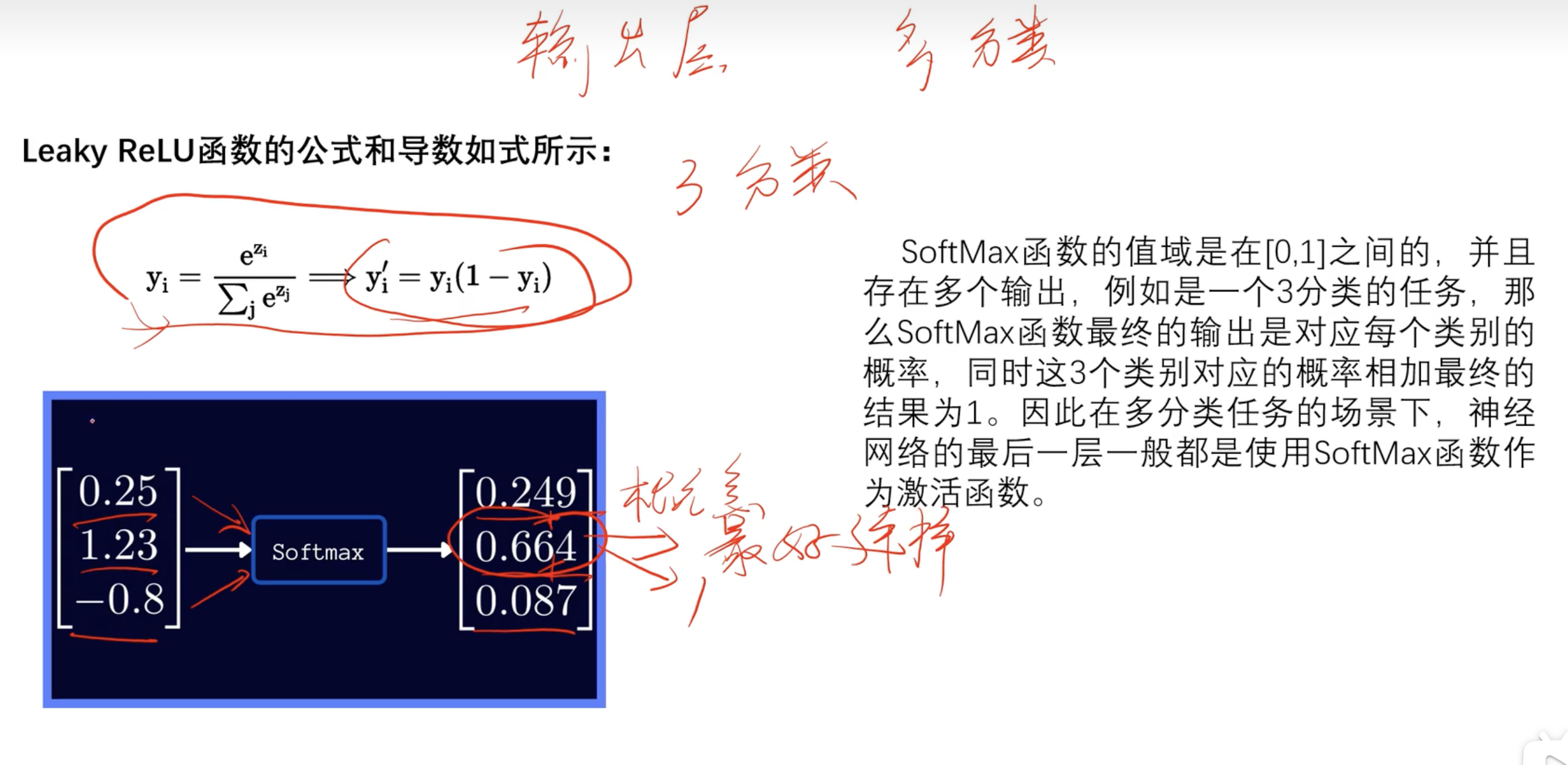
SoftMax

• 用于多分类任务
• 用于输出层

前向传播

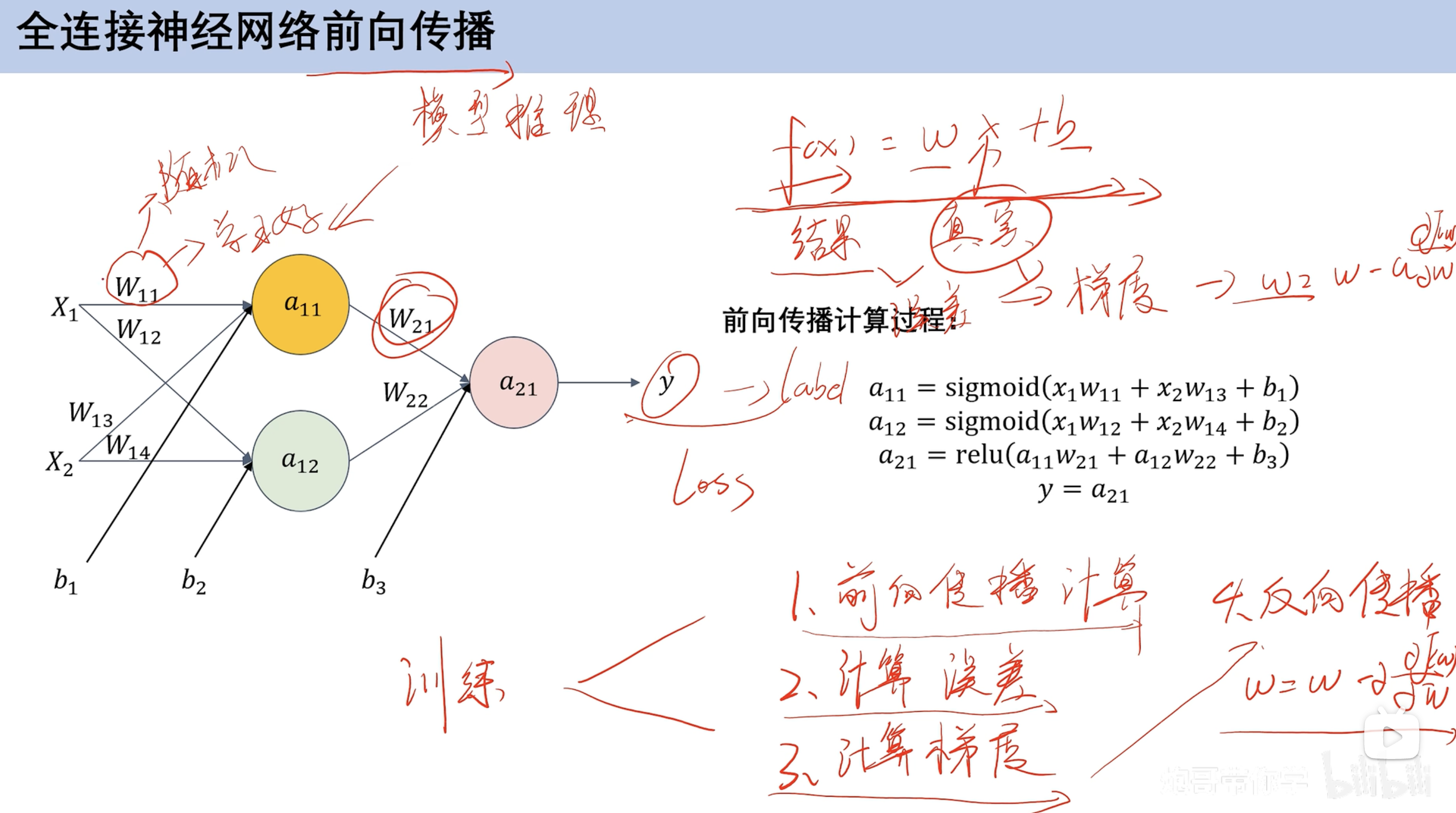
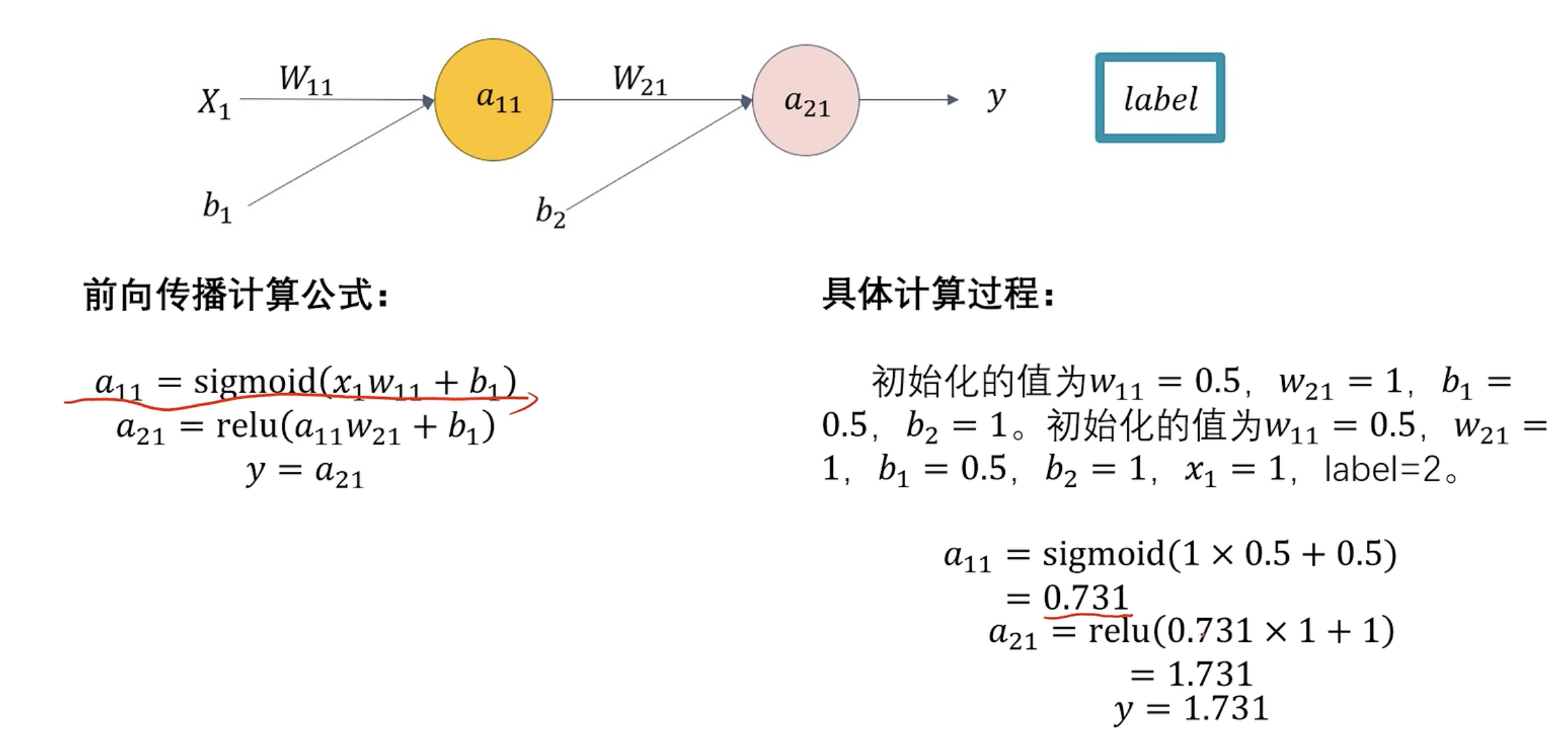
1. 前向传播计算 预设w和b 根据数据集计算
2. 计算误差 类比损失函数
3. 计算梯度 梯度更新 求损失函数偏导
4. 反向传播 反向更新w和b

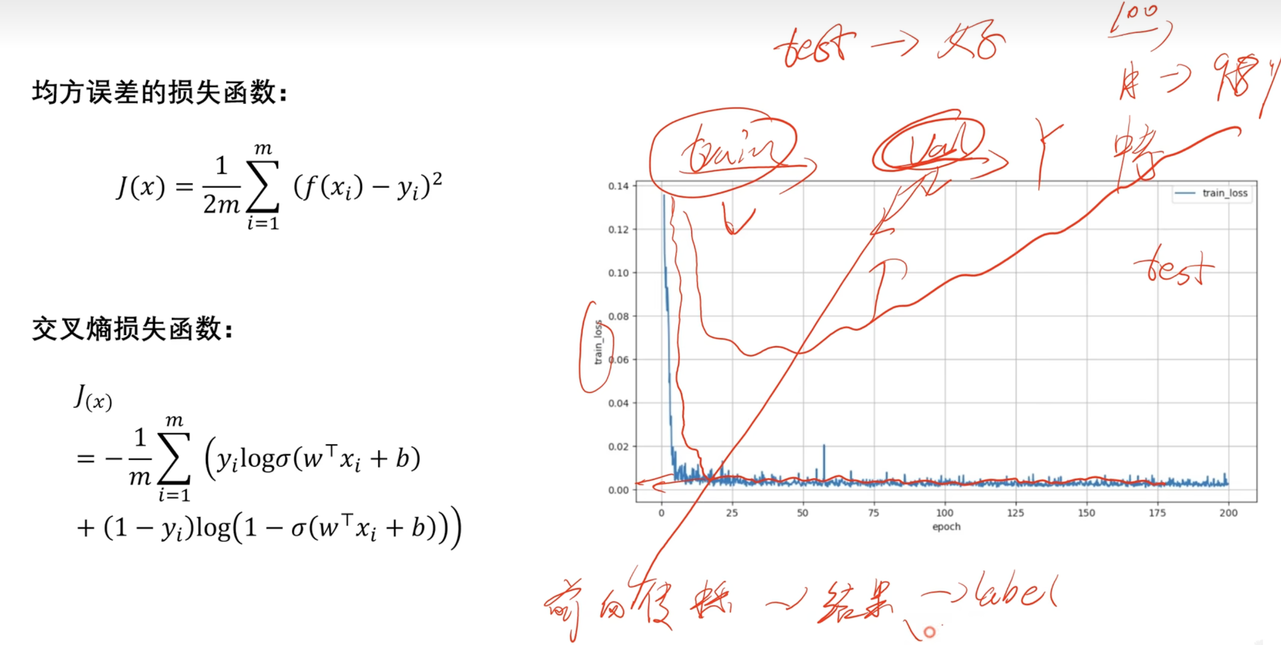
具体过程

损失函数

• 图像解释：前面cost值逐渐减小，w，b逐渐吻合，前向传播过程，用的train训练集

• 后面趋近于0 可能是测试集test

  

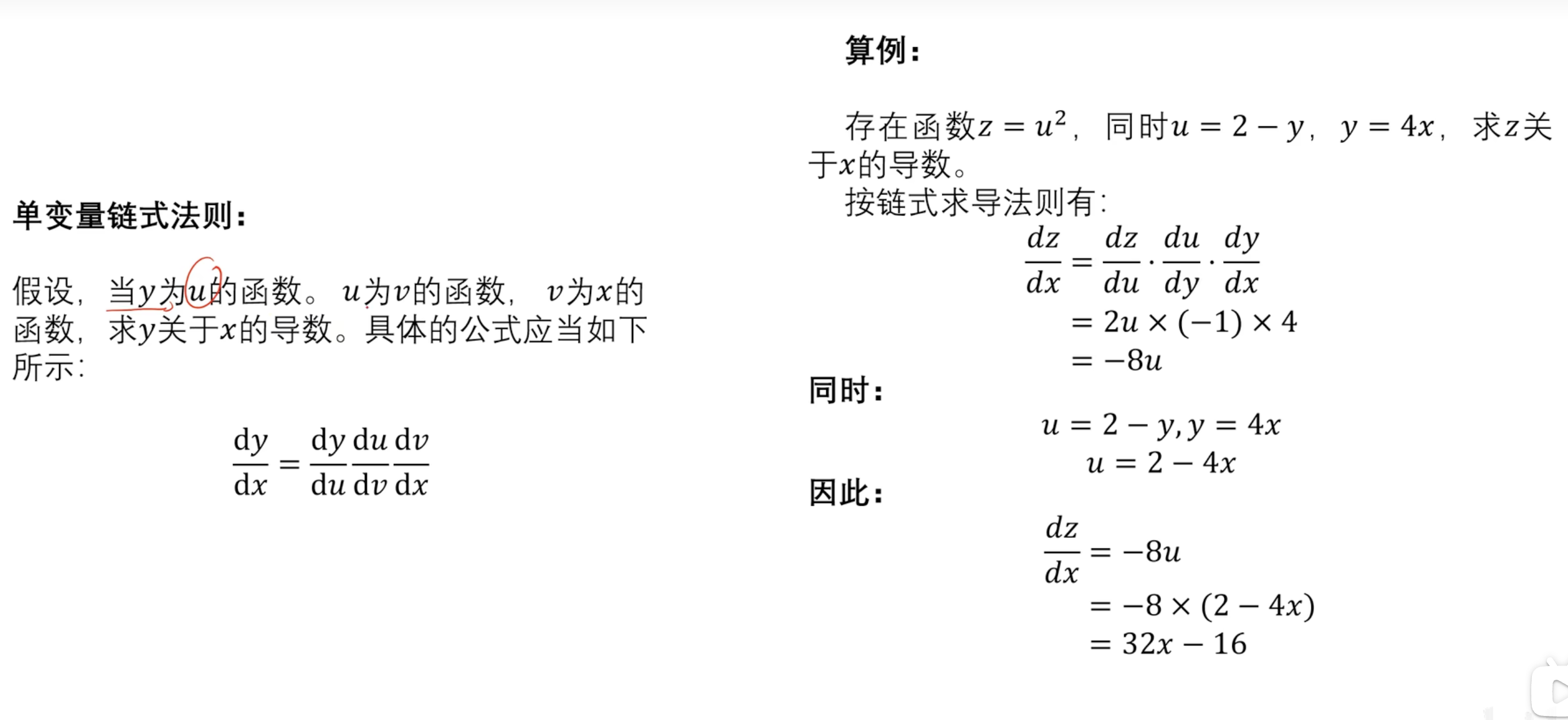
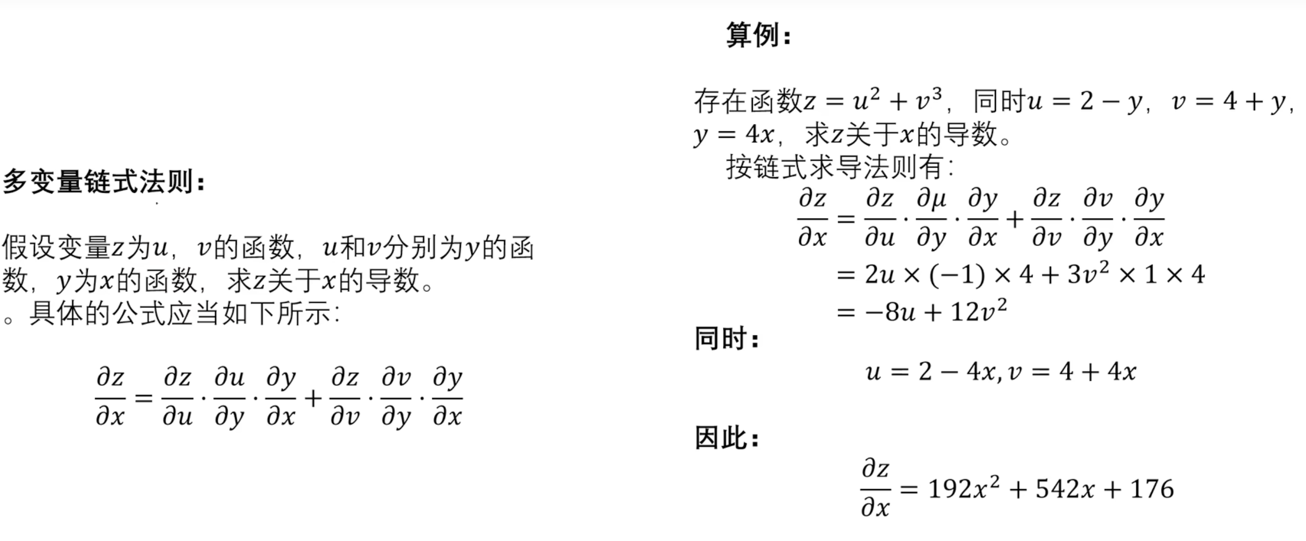
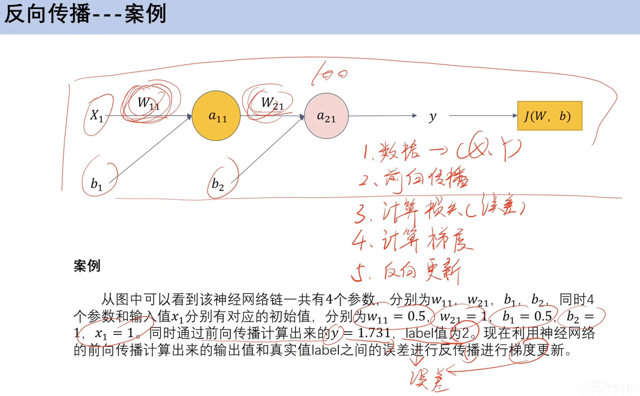
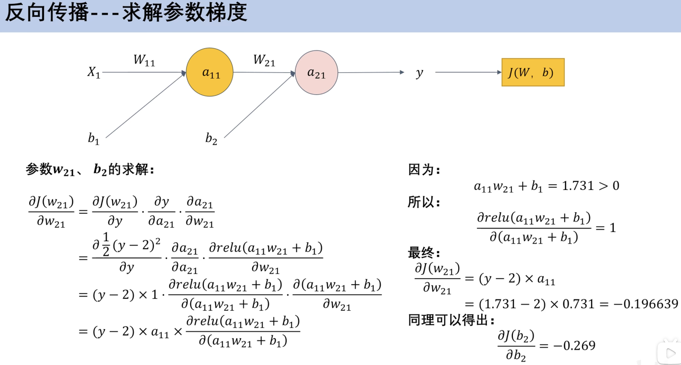
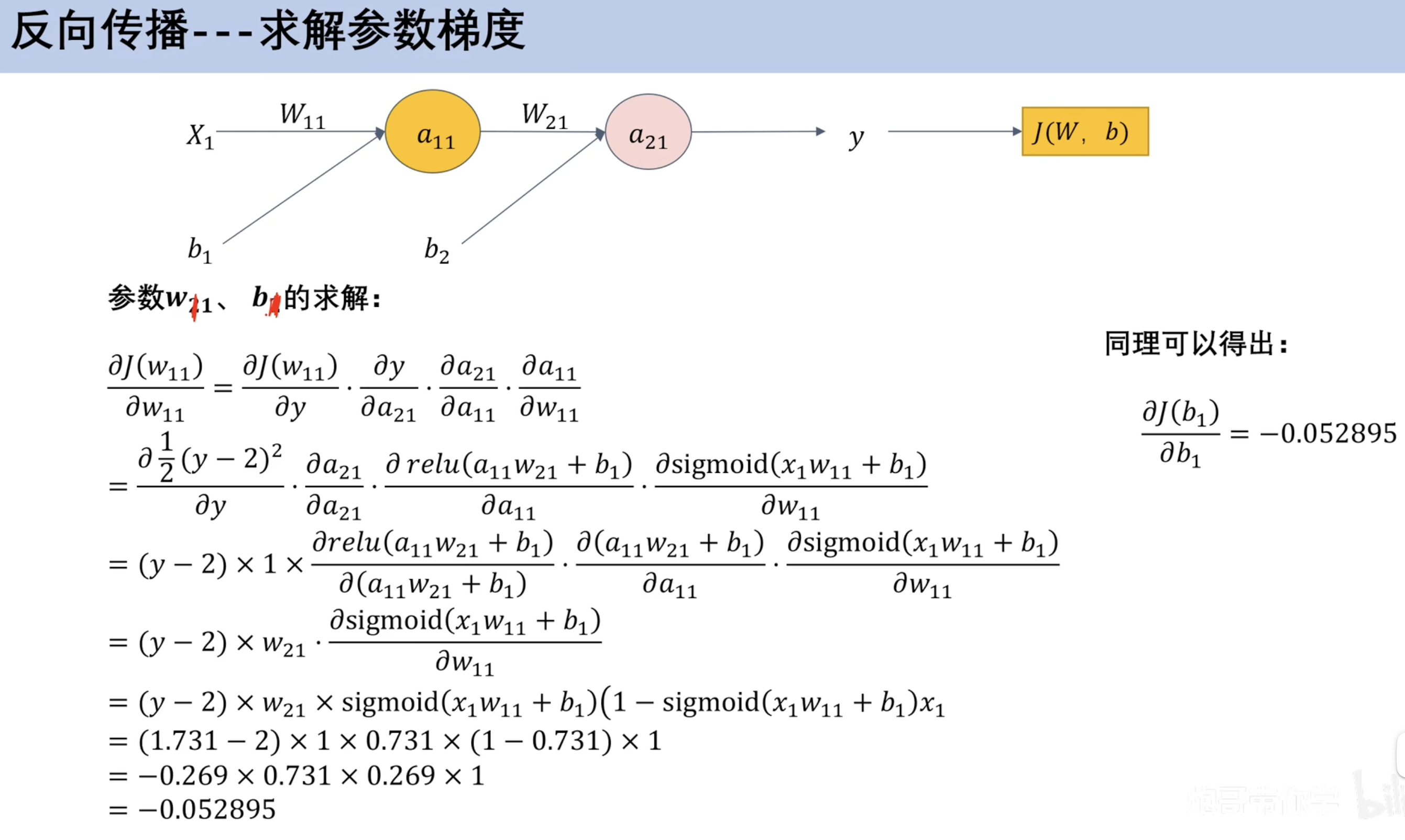
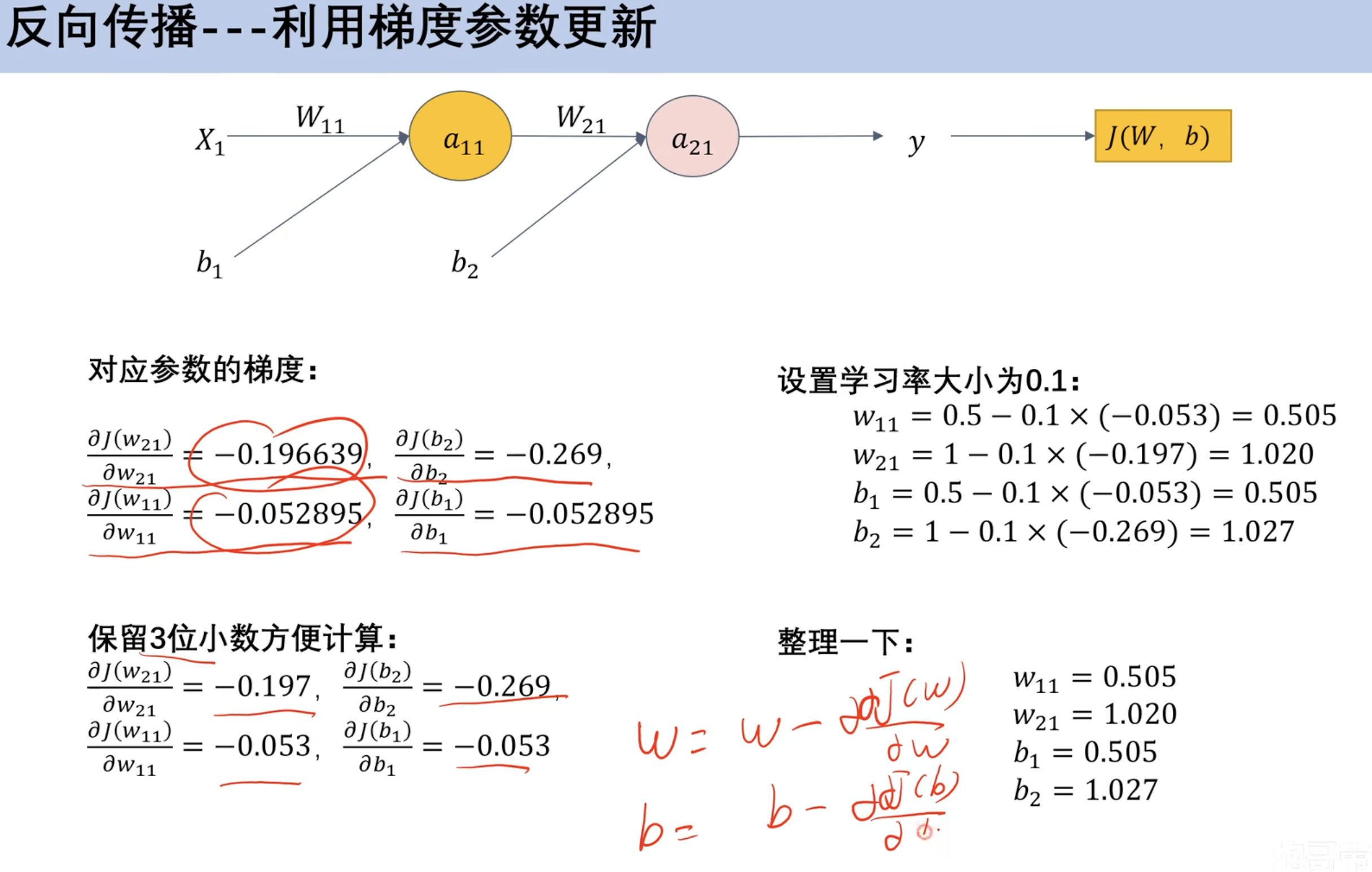
链式法则（数学补充）

单变量链式法则

多变量链式发展

==反向传播==

案例

求解参数梯度

利用梯度参数更新

• 设置学习率为0.1

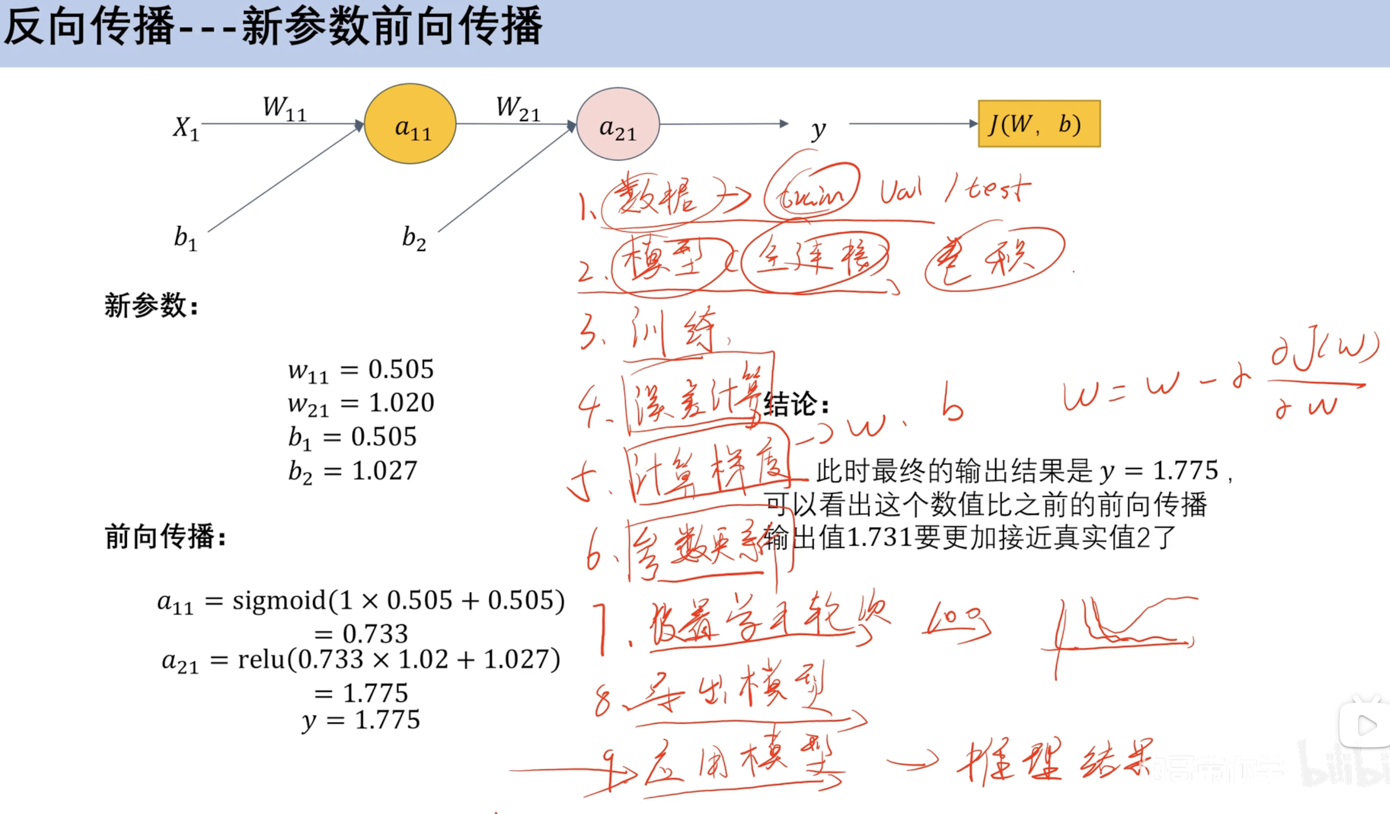
新参数前向传播

案例（预测乳腺癌 分类）

• 用全连接神经网络预测乳腺癌
• 对比机器学习

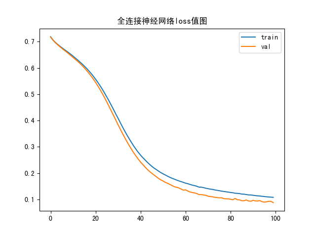
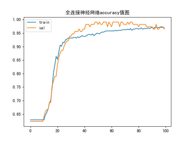
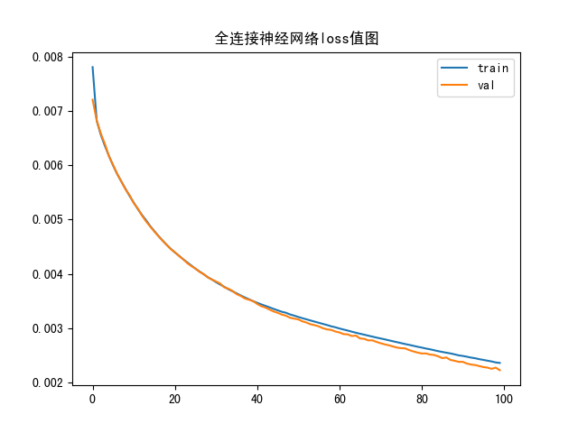
model_train

import numpy as np
import pandas as pd
import matplotlib.pyplot as plt
from sklearn.preprocessing import MinMaxScaler
from sklearn.model_selection import train_test_split
import keras
from keras.layers import Dense  # 稠密层
from keras.utils.np_utils import to_categorical
from sklearn.metrics import classification_report  # 验证
import matplotlib.font_manager as font_manager



# 解决中文显示问题
# font_path = '../SimHei.ttf'  # 将此路径替换为你自己的 SimHei 字体文件的实际路径，也就是刚刚第二步得到的那个路径
# font_manager.fontManager.addfont(font_path)
# plt.rcParams['font.sans-serif'] = ['SimHei']
# plt.rcParams['axes.unicode_minus'] = False

# 111111111111111111111111 数据预处理 1111111111111111111111111111111111111111111111
# 加载数据集
dataset = pd.read_csv("breast_cancer_data.csv")

# 提取特征和标签
X = dataset.iloc[:, :-1]
Y = dataset['target']

# 划分训练集和测试集 random_state随机种子固定 保证每次数据随机一样
x_train, x_test, y_train, y_test = train_test_split(X, Y, test_size=0.2, random_state=42)

# 将数据标签转为one-hot 独热向量格式
y_train_one = to_categorical(y_train, 2)  # 2个类别
y_test_one = to_categorical(y_test, 2)
# print(y_train_one)  # [1. 0.]

# 将数据特征归一化
sc = MinMaxScaler(feature_range=(0, 1))
x_train = sc.fit_transform(x_train)
x_test = sc.fit_transform(x_test)

# 22222222222222222222 用keras框架搭建深度学习神经网络模型 22222222222222222222222222222222222222222222
model = keras.Sequential()
model.add(Dense(10, activation='relu'))
model.add(Dense(10, activation='relu'))
model.add(Dense(2, activation='softmax'))

# 对神经网络进行编译 损失函数+评价指标
#  categorical_crossentropy：交叉熵
#  optimizer优化器:SGD随机梯度向量法
#  metrics：评价指标 准确率
model.compile(loss='categorical_crossentropy', optimizer='SGD', metrics=['accuracy'])

# epochs轮数
# batch_size一次多少个一起 并行
# verbose 2表示控制台可观察
# validation_data验证数据 用测试集验证 框架用于判断是否过拟合
history = model.fit(x_train, y_train_one, epochs=120, batch_size=64, verbose=2, validation_data=(x_test, y_test_one))
model.save('model.h5')

# 333333333333333333333 绘图 333333333333333333333333333333
plt.plot(history.history['loss'], label='train') # 训练集loss值
plt.plot(history.history['val_loss'], label='val') # 验证集loss值
plt.title("全连接神经网络loss值图")
plt.legend() # 图例
plt.show()

# 绘制训练集和验证集的准确率对比图
plt.plot(history.history['accuracy'], label='train') # 训练集准确率
plt.plot(history.history['val_accuracy'], label='val') # 验证集准确率
plt.title("全连接神经网络accuracy值图")
plt.legend() # 图例
plt.show()

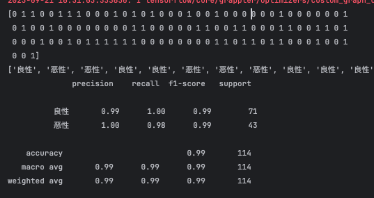
model_test

from cProfile import label

import numpy as np
import pandas as pd
import matplotlib.pyplot as plt
from sklearn.preprocessing import MinMaxScaler
from sklearn.model_selection import train_test_split
import keras
from keras.layers import Dense  # 稠密层
from keras.utils.np_utils import to_categorical
from sklearn.metrics import classification_report  # 验证
import matplotlib.font_manager as font_manager
from keras.models import load_model

# 111111111111111111111111 数据预处理 1111111111111111111111111111111111111111111111
# 加载数据集
dataset = pd.read_csv("breast_cancer_data.csv")

# 提取特征和标签
X = dataset.iloc[:, :-1]
Y = dataset['target']

# 划分训练集和测试集 random_state随机种子固定 保证每次数据随机一样
x_train, x_test, y_train, y_test = train_test_split(X, Y, test_size=0.2, random_state=42)

# 将数据标签转为one-hot 独热向量格式
y_test_one = to_categorical(y_test, 2)
# print(y_train_one)  # [1. 0.]

# 将数据特征归一化
sc = MinMaxScaler(feature_range=(0, 1))
x_test = sc.fit_transform(x_test)

# 导入模型
model = load_model("model.h5")

# 利用训练好的模型进行测试
predict = model.predict(x_test)
# print(predict)

y_pred = np.argmax(predict, axis=1)
print(y_pred)  # [0,1,0]

# 转为汉字
result = []
for i in range(len(y_pred)):
    if y_pred[i] == 0:
        result.append("良性")
    else:
        result.append("恶性")
print(result)

# 打印模型精确到 召回率
report = classification_report(y_test, y_pred, labels=[0, 1], target_names=["良性", "恶性"])
print(report)

函数图像

loss

accuracy

预测报告

案例（空气质量 线性回归）

model_train

import numpy as np
import pandas as pd
import matplotlib.pyplot as plt
from sklearn.preprocessing import MinMaxScaler
from sklearn.model_selection import train_test_split
import keras
from keras.layers import Dense  # 稠密层
from keras.utils.np_utils import to_categorical

#  11111111111111111111111111 数据处理 1111111111111111111111
# 导入数据
dataset = pd.read_csv("data.csv")

# 将数据归一化
sc = MinMaxScaler(feature_range=(0, 1))
scaled = sc.fit_transform(dataset)  # 数列形式 没有列名

# 将归一化数据转为dataframe格式，方便后续处理
dataset_sc = pd.DataFrame(scaled)  # 有类名 同dataset
print(dataset_sc)

# 找出特征值和标签
X = dataset_sc.iloc[:, :-1]  # 所有行除了最后一列
Y = dataset_sc.iloc[:, -1]  # 所有行 最后一列

x_train, x_test, y_train, y_test = train_test_split(X, Y, test_size=0.2, random_state=42)

# 22222222222222222222222 利用keras模型搭建 2222222222222222222222222222222222
model = keras.Sequential()
model.add(Dense(10, activation='relu'))
model.add(Dense(10, activation='relu'))
model.add(Dense(1))  # 输出层 不要激活函数 但要反归一化

# 对神经网络进行编译
model.compile(loss='mse', optimizer='SGD')

# 模型训练
history = model.fit(x_train, y_train, epochs=100, batch_size=32, verbose=2, validation_data=(x_test, y_test))
model.save('model.h5')

# 333333333333333333 可视化 3333333333333333
plt.plot(history.history['loss'], label='train')
plt.plot(history.history['val_loss'], label='val')
plt.title("全连接神经网络loss值图")
plt.legend()
plt.show()

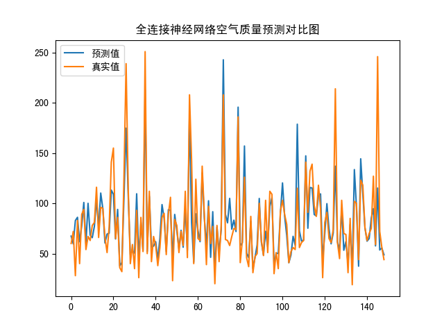
model_test

import numpy as np
import pandas as pd
import matplotlib.pyplot as plt
from scipy.ndimage import label
from sklearn.preprocessing import MinMaxScaler
from sklearn.model_selection import train_test_split
import keras
from keras.layers import Dense  # 稠密层
from keras.utils.np_utils import to_categorical
from keras.models import load_model
from math import sqrt
from numpy import concatenate
from sklearn.metrics import mean_squared_error

#  11111111111111111111111111 数据处理 1111111111111111111111
# 导入数据
dataset = pd.read_csv("data.csv")

# 将数据归一化
sc = MinMaxScaler(feature_range=(0, 1))
scaled = sc.fit_transform(dataset)  # 数列形式 没有列名

# 将归一化数据转为dataframe格式，方便后续处理
dataset_sc = pd.DataFrame(scaled)  # 有类名 同dataset

# 找出特征值和标签
X = dataset_sc.iloc[:, :-1]  # 所有行除了最后一列
Y = dataset_sc.iloc[:, -1]  # 所有行 最后一列

x_train, x_test, y_train, y_test = train_test_split(X, Y, test_size=0.05, random_state=42)

# 2222222222222 加载训练好的模型 222222222222222222
model = load_model("model.h5")

# 预测
yhat = model.predict(x_test)
# print(yhat) # [0.1681547 ]

# 预测值反归一化
inv_yhat = concatenate((x_test, yhat), axis=1) # 连接两个Numpy数据
# print(inv_yhat) # 归一数据 [0.05119454 0.09076175 0.06796117 ... 0.14107884 0.56149733 0.13507885]
inv_yhat = sc.inverse_transform(inv_yhat) # 反归一化
# print(inv_yhat)  [ 12.          24.           5.         ...   1.57         7.
#    82.83994955]
prediction = inv_yhat[:, 6]
# print(prediction)

# 将y_test维度转换 二维
# 2396    0.117073
# 1407    0.146341
y_test = np.array(y_test) # [0.11707317 0.14634146]
y_test = np.reshape(y_test, (y_test.shape[0], 1)) # [[0.11707317 0.14634146]]

# 反向缩放真实值
# print(x_test) # 2396  0.051195  0.090762  0.067961  0.172414  0.141079  0.561497
inv_y = concatenate((x_test, y_test), axis=1)
print(inv_y)
inv_y = sc.inverse_transform(inv_y)
real = inv_y[:, 6]
print(real)

# 333333333333333 评价 333333333333333333
# 计算rmse和MAPE
remse = sqrt(mean_squared_error(real, prediction))
mape = np.mean(np.abs(real - prediction) / real)
print("remse", remse)
print("mape", mape)

# 画出真实值和预测值对比图
plt.plot(prediction, label="预测值")
plt.plot(real, label="真实值")
plt.title("全连接神经网络空气质量预测对比图")
plt.legend()
plt.show()

loss图像

真实值预测值对比图